Jekyll2026-04-12T22:27:23+00:00https://brianhliou.com/feed.xmlBrian LiouI build backend systems and side projects. Writing about technical things and other stuff I'm thinking about.Brian Liouhttps://brianhliou.comThe Market Isn’t One Game2026-03-28T00:00:00+00:002026-03-28T00:00:00+00:00https://brianhliou.com/posts/the-market-isnt-one-gamePeople explain why you can’t beat the market in two ways. Either it’s rigged, or you’re not smart enough. Both miss the point.
The real problem is that the market isn’t one game. It’s a bunch of different games happening at the same time, on the same board, with the same pieces, but under completely different rules depending on who you are. Most people don’t lose because they play badly. They lose because they don’t realize which game they’re in.
Why This Is Harder Than Any Other Game
Every competitive game humans have come up with is simpler than markets. Chess has about 20 moves per turn. Go has about 250. Real-time games like League of Legends add execution pressure, fog of war, and team coordination on top of that.
Markets are past all of them. Four things make them different.
The game rewrites itself. A strategy that works attracts money. More money changes prices. Changed prices kill the strategy. In chess, no move you make changes the rules of chess. In markets, the rules shift based on how people play. The game mutates in response to its own players.
You never see the full board. In Go, both players can see everything. In markets, the relevant information includes geopolitics, weather, psychology, corporate fraud, central bank policy, and whatever is happening in a CEO’s personal life. Most of it is hidden, delayed, or just wrong.
You can’t see your opponents. The other side of your trade could be a retiree moving money around, a hedge fund closing a position, or an insider who already knows what’s about to happen. You don’t pick who you play against and you can’t tell how good they are.
There’s no finish line. You can’t get checkmated. There’s no final score. Which means losses can always become “I’m just early.” Every other game ends. This one doesn’t.
Complexity scale:

Chess → Poker → Go → League of Legends → Markets
 20        ~5    250    real-time +           all of
moves/   hidden  moves/  fog of war +        the left +
turn     cards   turn    coordination        reflexivity +
                                             infinite players +
                                             no win condition
Six Games, One Board
Here’s the framework. The market isn’t one game with a skill ladder. It’s six different games being played in the same place. And they stack. Each one above requires something the one below doesn’t have.
┌─────────────────────────────────────────────────┐
│  ACCESS        Insider knowledge, connections    │ ← information you shouldn't have
├─────────────────────────────────────────────────┤
│  STRUCTURAL    Market making, HFT, liquidity    │ ← co-located servers, exchange access
├─────────────────────────────────────────────────┤
│  SIGNAL        Proprietary data → predictions   │ ← alt-data pipelines, ML at scale
├─────────────────────────────────────────────────┤
│  SYSTEMATIC    Quant process, factor exposure   │ ← tooling, discipline, AI-augmented research
├─────────────────────────────────────────────────┤
│  ANALYTICAL    Fundamental research, valuation  │ ← domain knowledge, time
├─────────────────────────────────────────────────┤
│  NARRATIVE     Vibes, sentiment, stories        │ ← a brokerage account
└─────────────────────────────────────────────────┘
  Each level up requires new data, infrastructure, or capital to unlock.
Game
What the edge is
What you need to unlock it
Narrative
Sentiment, vibes, stories
A brokerage account and an opinion
Analytical
Better understanding of what a business is worth
Domain knowledge, financial literacy, time to research
Systematic
Quantitative process, run at scale
Tooling, programming ability, discipline to follow a process
Signal
Proprietary data turned into predictions
Alt-data pipelines, ML infrastructure, serious capital for data acquisition
Structural
Profiting from how markets work, not from predicting prices
Each level up isn’t just harder. It requires something fundamentally different. You don’t graduate from Analytical to Systematic by getting smarter. You need different tools, different infrastructure, and often different capital. A jogger doesn’t become a Formula 1 driver by running faster. They need a completely different vehicle.
Getting better at the Narrative game will never get you the returns available in the Signal game. Picking the wrong game costs you more than playing your game badly.
Above the Game
Some players aren’t even competing for returns. They run the arena.
┌───────────────────────────────────┐
│  SOVEREIGNS                       │  Can flip the table
│  (nation-states, SWFs)            │
├───────────────────────────────────┤
│  RULE-SETTERS                     │  Write the rules
│  (Fed, SEC, regulators)           │
├───────────────────────────────────┤
│  INFRASTRUCTURE                   │  Tax every transaction
│  (exchanges, index providers)     │
├───────────────────────────────────┤
│  ┌─────────────────────────────┐  │
│  │      THE SIX GAMES          │  │  Compete for returns
│  │    (all the players)        │  │
│  └─────────────────────────────┘  │
└───────────────────────────────────┘
Infrastructure takes a cut of every transaction. Exchanges, clearinghouses, index providers, data vendors. When S&P adds a stock to an index, billions of dollars move automatically. These players don’t need to be right about anything. They just collect rent.
Rule-setters decide the rules everyone else is trying to model. The Fed doesn’t predict interest rates. It decides them. When the SEC approved Bitcoin ETFs, hundreds of billions in new flows opened up overnight. One regulatory decision can create or wipe out an entire market.
Sovereigns can flip the whole table. Sanctions, capital controls, currency interventions. A sovereign wealth fund can move a market just by showing up or leaving.
The higher up this stack you go, the less skill matters. These players don’t play the game. They shape the board.
Marked Cards
Then there are insiders. They break the whole framework because they’re not playing better. They already know the answer.
Hard insiders are corporate officers and deal advisors trading on information that isn’t public yet. Illegal. Sometimes prosecuted. Soft insiders are people like engineers who can feel demand shifting before it hits earnings, or lobbyists who know which way a regulation is going, or VCs who see private metrics that tell you where public markets are headed. Mostly legal, definitely gray. Political insiders are legislators trading on policy knowledge. The STOCK Act makes it illegal. Nobody enforces it. Connected capital isn’t inside the room, but close enough to the room that information leaks to them through relationships. You can see this in the unusual options activity that shows up before almost every big acquisition. Somebody always knows.
These people haven’t found a better chess move. They’ve read the last page of the book. And they make the game harder for everyone else, because some of what looks like random market movement is actually people trading on things that haven’t been announced yet.
The Index Paradox
Given everything above, here’s the strangest part. The best move for most players is to stop playing.
An index fund has no strategy. It holds everything. It doesn’t think. It beats the majority of active participants because it has no research costs, almost no transaction costs, never panics, and captures the economic return of owning businesses without trying to compete.
No other game works like this. There’s no chess equivalent of “don’t play, collect the average score of everyone, and beat 80% of them.” In markets that’s a real option and it works.
This sets the floor. Whatever you do, you have to beat this. Not just make money. Make more than you would have made doing literally nothing. After trading costs, after taxes, after the time you spent thinking about it.
What’s the Highest Level You Can Actually Play?
This is the question the whole framework builds toward.
Look at the stack again. Access requires connections you probably don’t have. Structural requires exchange infrastructure and regulatory approvals. Signal requires millions in data acquisition and ML infrastructure.
For most individuals, the realistic ceiling is the Systematic game. You need programming ability, good tooling, and the discipline to follow a quantitative process. That’s a real unlock, but it’s an unlock most technically skilled people can actually reach.
AI shifts the ceiling here. One person with good tooling can now chew through earnings transcripts, SEC filings, patent data, job postings, and alternative data at a throughput that would have cost seven figures in analyst salaries five years ago. The edge isn’t some superhuman insight. It’s coverage. You can look at more things more consistently than any single human analyst.
But the ceiling of that game is specific. You’re hunting for mispricings in places where big money can’t go without moving prices. Micro-caps, weird special situations, post-spinoff equities, niche sectors with almost no analyst coverage. Your edge is that the space is too small and too annoying for institutional capital to bother with.
So what can you actually make?
Honestly, a few percentage points over the index per year. Sustained over a long time. With real variance and stretches where you underperform and wonder if the whole thing is broken.
Not 60%+ annual returns like Renaissance’s Medallion fund. Those come from the Signal and Structural games at a scale and speed you can’t touch as a solo player.
Realistic annual returns by game:

Narrative:     negative after costs (most retail traders lose money)
Analytical:    roughly index-matching after effort and fees
Systematic:    index + 2-5% in favorable conditions, with dry spells
Signal:        10-30%+ (requires massive infrastructure investment)
Structural:    consistent but requires institutional setup
Access:        high, but illegal or ethically gray

Index fund:    7-10% long-term average, no effort, no skill required
The index does about 7-10% a year over long periods. To justify playing actively, you need to clear that plus trading costs, tax drag, and the value of the time you’re spending. A good systematic solo player might compound at 12-15% in a good environment. That’s real money over decades. But it demands:
A specific theory of your edge that you could be proven wrong about. Not “I’m smart.” Something like “I find micro-cap spinoffs before institutional coverage shows up.”
A process that works without you needing to feel inspired or convicted in the moment
Position sizing where no single mistake can blow you up
The ability to watch yourself underperform the index for years and keep going anyway
Most of the edge available at this level comes from going where the market doesn’t look. Your advantage is the hassle. The day it stops being a hassle for bigger players, the advantage disappears.
How to Think About All This
A few things fall out of the framework.
The market isn’t your opponent. It’s the combined output of everyone playing every game at once. Beating it means beating the weighted average of all of them, including the majority who lose. The bar is lower than it sounds, but higher than most people clear.
The first decision is which game to play. Not which stock to buy. Which game. Most people never think about this consciously. The game gets chosen for them. Usually it’s the Narrative game, which has the worst expected returns of all six.
Each game above requires a new unlock. You don’t level up by getting smarter at your current game. You level up by acquiring something new: tooling, data, infrastructure, access. If you don’t have what the next level requires, you can’t play it no matter how skilled you are.
The ceiling is real. For a solo player, the Systematic game is as high as it goes. The returns there are meaningful but not spectacular. A few points of alpha over long periods. The Signal, Structural, and Access games pay better but require things individuals don’t have.
Indexing is the right default. Not because the game can’t be beaten. It can. But knowing whether you can beat it is itself an incredibly hard problem. Everyone thinks they’re above average. The cost of being wrong is years of underperformance plus all the time you spent. The “just index” advice isn’t giving up. It’s the right answer for most people in a game where you can’t reliably judge your own skill level.
The most important question isn’t whether the market can be beaten. It’s whether you can honestly figure out which game you’re playing and whether your edge in that game is real enough to clear the index after all costs. If you can’t answer that clearly, the answer is already index.
The next question is what actually happens when you try to play the Systematic game for real. That’s what I’m building toward.
What You Learned
✓ Markets are six different games on one board, not one game with skill levels
✓ Each game above requires new data, infrastructure, or capital to unlock
✓ Picking the wrong game costs more than playing your game badly
✓ The highest realistic level for a solo player is the Systematic game
✓ The honest return ceiling there is a few points of alpha per year, with long dry spells
✓ Indexing is the right default because self-assessment in this game is unreliable
Renaissance Technologies - Background on the most successful quant fund, playing the Signal game at its peak
Annie Duke - Author of Thinking in Bets, on making decisions when you can’t know the outcome
Unusual Whales - Tracks congressional trading, real data on the Access game
]]>Brian Liouhttps://brianhliou.comI Built an AI System That Synthesizes Stock Intelligence2026-03-09T00:00:00+00:002026-03-09T00:00:00+00:00https://brianhliou.com/posts/signal-rundownEvery analyst has an opinion on the market. Almost none of them show you the data behind it, update it as new information comes in, or tell you when they were wrong.
The problem with market analysis today isn’t a lack of information. It’s a lack of synthesis. There are dozens of sources covering any major stock: earnings reports, insider trades, analyst ratings, SEC filings, news articles. Nobody’s reading all of them. And the analysts who do form opinions rarely tie them to specific, timestamped, falsifiable claims.
I wanted to test something: if you point AI at the full firehose of financial news and force it to take structured positions backed by specific data, can it produce better intelligence than reading five articles? So I built a system to find out.
Signal Rundown is an AI that reads dozens of financial sources every 2 hours, maintains explicit bullish/bearish/neutral positions on every stock it tracks, and surfaces the data behind each call. Insider trades, analyst ratings, earnings data, direction changes, all synthesized into what actually matters.
What It Actually Does
Signal Rundown is not a chatbot and not a news aggregator. It’s a signal extraction and synthesis system that runs continuously.
Every 2 hours, the system pulls from dozens of sources (RSS feeds, Google News, financial data APIs) and filters aggressively, because most financial news is noise. The articles that survive get their full text extracted and run through LLMs that break each one down into structured signals: direction, key facts, sentiment, which companies are affected.
This matters because raw articles are ambiguous. A single earnings report might be bullish for the company, bearish for a competitor, and neutral for the sector. The extraction step forces a position.
Those signals accumulate into entity states: a rolling analytical position per stock that updates as new evidence arrives. Each entity state includes a direction, a headline thesis, the key data points driving the call, and what to watch next. When a major event approaches, like earnings, the system generates predictions with a specific direction, baseline price, and expected move range.
The tech stack is Python, PostgreSQL, and LLMs. The whole system runs on a single Railway instance for about $30/month. Collection happens every 2 hours from 5 AM, entity states update on the same cadence, and the dashboard updates continuously.
What Makes It Different
Most analysis is stateless. Someone publishes a take, it floats around for a day, and it’s forgotten. Nobody checks whether it was right.
Signal Rundown works more like a real analyst: it maintains views, updates them as evidence changes, and shows you exactly what data drove each position. Every entity has a living analytical state that accumulates evidence over time. When the system flips from bullish to bearish, that shift is logged with the specific signals that caused it.
The difference is synthesis at scale. Signal Rundown does this across dozens of stocks simultaneously, processes information in minutes instead of days, and never has a bad Monday. For each stock, you see not just “bullish” or “bearish” but the insider trades, analyst ratings, earnings data, and news signals that support the call.
The other key decision: predictions are first-class objects, not chat responses. Each prediction records a baseline price, an expected move range, and a target event. After the event, the system scores the prediction against the actual price. The track record is public and permanent.
What It Looks Like
The system has been running in production for several weeks. Each entity page shows the AI’s full analytical state: direction, key data points, what to watch, insider activity, analyst consensus, and active predictions.
Here’s an example of the social card the system generates for NVDA:
That’s not a summary of one article. That’s the synthesis of dozens of signals from multiple sources, updated every 2 hours. The system spotted the insider selling pattern, cross-referenced it with the margin data, and formed a view.
What’s Next
Two things I’m focused on:
Building the track record. The prediction system is live and scoring against real prices. As more events get scored, the accuracy data will speak for itself. I’ll publish results when there’s enough data to be meaningful.
]]>Brian Liouhttps://brianhliou.comBuilding a Model Serving API From Scratch2026-02-22T00:00:00+00:002026-02-22T00:00:00+00:00https://brianhliou.com/posts/model-serving-apiI built a model serving API from scratch. Not because the world needs another inference server, but because I wanted to understand what happens between “send prompt” and “receive tokens.” The things ML system design interviews ask about: batching, backpressure, streaming, graceful degradation. I wanted hands-on experience so I could talk about them from building, not reading.
The result: a FastAPI server wrapping Ollama with a bounded request queue, SSE streaming, naive batching, 11 custom Prometheus metrics, and structured logging. It runs on a $7/month ARM server. I ran 8 structured experiments against it. The data revealed things I didn’t expect.
Four containers on a single machine. Caddy terminates TLS with automatic Let’s Encrypt certificates (three lines of config). FastAPI handles the serving logic: bounded request queue, batch dispatcher, OpenAI-compatible API, Prometheus metrics. Ollama wraps llama.cpp and runs the model. Grafana Alloy scrapes metrics every 15 seconds and ships them to Grafana Cloud.
The containers communicate over a Docker bridge network using service names as hostnames. Caddy resolves api, FastAPI resolves ollama, Alloy resolves api. Sub-millisecond latency between containers because the traffic never leaves the host. Only Caddy exposes ports to the internet (80, 443). The FastAPI port binds to 127.0.0.1 only.
The core idea: a bounded request queue sits between clients and the model. When the queue is full, clients get an instant 503 with Retry-After instead of waiting indefinitely. This is backpressure: the serving layer’s most important job.
The API is OpenAI-compatible (/v1/chat/completions), supports streaming via SSE, and exposes 11 custom Prometheus metrics (TTFT, tokens/sec, queue depth, error rates by type, backend latency).
What the model actually does
The model running on this server is Llama 3.2 3B Instruct: 3.21 billion parameters, 28 transformer layers, 128K token context window. It was built through knowledge distillation from Meta’s larger Llama 3.1 8B and 70B models. The 3B model wasn’t trained from scratch. Instead, Meta pruned the 8B architecture down to 3B parameters, then trained the smaller model to match the output distributions of the larger ones. This is why a 3B model performs competitively with many 7B models.
How a single token is generated
When you send “What is 2+2?” to the API, the model processes it through 28 identical transformer layers. Each layer does two things:
Attention: The model decides which parts of the input matter for predicting the next word. For each position, it computes query, key, and value vectors, calculates attention scores between all positions, and produces a weighted sum. Llama 3.2 uses Grouped Query Attention (GQA): 24 query heads share 8 key-value heads (a 3:1 ratio). This cuts the memory needed for cached attention data by 3x.
Feed-forward network: Each token’s representation passes through a gated network (SwiGLU) with three weight matrices: gate, up, and down projections. The gate controls information flow through element-wise multiplication. Each FFN layer has ~75 million parameters.
After all 28 layers, the model produces a probability distribution over 128,256 possible tokens. Temperature scaling adjusts how “random” the selection is (lower = more deterministic), and top-p sampling filters the candidate set. One token is drawn from this distribution.
This entire process repeats for every single output token, one at a time.
Two-phase inference
Token generation has two distinct phases with very different performance characteristics:
Prefill (prompt processing): All input tokens are processed in parallel through the transformer. This is compute-bound: lots of matrix multiplications that can be parallelized across CPU cores. Speed: 50-150+ tokens/second.
Decode (generation): Each output token is generated sequentially. The model must read its entire 2 GB of weights from memory to produce one token. This is memory-bandwidth-bound: the CPU can compute faster than it can load data. Speed: 7-8 tokens/second.
The decode bottleneck explains a key number in my experiments. To generate one token, the CPU reads ~2 GB of model weights from RAM. With the server’s DDR4 memory bandwidth, the theoretical ceiling is roughly 15-30 tokens/second. After overhead from the KV cache, dequantization, and non-sequential memory access, the practical rate is ~7.5 tok/s. This rate is nearly identical whether the system is idle or under heavy load.
How a 3B model fits in 8GB RAM
The raw model weights in 16-bit precision would be 6.4 GB. That doesn’t fit. Ollama uses Q4_K_M quantization: weights are compressed from 16 bits to ~4.5 bits per parameter by clustering weight values into discrete bins using k-means. Sensitive layers (attention output, FFN down projection) get 5-6 bits; less sensitive layers get 4 bits.
The memory budget on this server:
Component
RAM
Model weights (Q4_K_M)
~2.0 GB
KV cache (inference state)
~0.5-1.0 GB
FastAPI + Python runtime
~100 MB
Caddy + Alloy + Docker
~200 MB
OS + kernel
~300 MB
Total active
~3.1-3.6 GB
Page cache (remaining)
~4.4-4.9 GB
Comfortable margin. The KV cache stores attention keys and values from all previous tokens so the model doesn’t recompute them. Each token in the cache costs 112 KB across all 28 layers and 8 KV heads. At 2K context, that’s ~224 MB. At 8K, ~900 MB. At the model’s full 128K context, the KV cache alone would need ~14 GB, which is why CPU inference practically limits context length.
Backpressure works, but the math is brutal
I sent 100 simultaneous requests against a queue of 50:
Outcome
Count
Rejected instantly (503)
50
Accepted, then timed out (504)
50
Successful (200)
0
Zero successful completions. Not one.
Ollama processes requests sequentially. Each request takes 2-3 seconds. 50 queued requests need 100-150 seconds to drain. The request timeout is 60 seconds. So by the time the server gets to request #26, the deadline has already passed.
The queue protects the system from crashing. Rejected clients get an instant response and can retry. But the queue doesn’t make the system faster. A queue of 50 with a sequential backend and 60s timeout means accepting work you can’t finish.
The correct formula: max_queue_size = (timeout / avg_request_duration) * backend_concurrency. For this system: 60s / 2.5s * 1 = 24. My queue of 50 is too large.
The “queue” isn’t really a queue
Looking deeper at the implementation, QueueManager is not a FIFO queue. It’s a counter. There’s no asyncio.Queue, no waiting, no ordering. When acquire() is called, it checks if active >= max_size. If yes, it immediately raises QueueFullError. If no, it increments the counter. That’s it. No mutex needed because asyncio is single-threaded.
This is actually a load shedder, not a queue. Requests are either admitted instantly or rejected instantly. The name “queue” is misleading. In the backpressure flood experiment, asyncio task scheduling, not arrival order, determined which requests got admitted. Request #0 (the first to arrive) was rejected while request #1 got in.
503 rejection isn’t fast enough
The 50 rejected requests averaged 0.87 seconds to get their 503 response. That’s nearly a full second to say “no.” For a fast-fail mechanism, that’s too slow.
The latency comes from the network stack: TLS handshake to the server, HTTP request parsing, response propagation back through Caddy. Under extreme load (100 simultaneous requests), the server’s event loop is contended. At concurrency 60 in another experiment, 503 rejections took only 0.73 seconds. The 140ms difference reflects the server being less overloaded.
Latency doesn’t just increase. It cliffs.
I swept concurrency from 1 to 60:
Concurrency
Avg Latency
Success Rate
1
7.4s
100%
2
4.3s
100%
5
10.0s
100%
10
18.7s
100%
20
42.9s
100%
30
20.9s
27%
50
43.7s
16%
60
39.2s
20%
The jump from 20 to 30 is the interesting part. Latency drops from 42.9s to 20.9s, but success rate craters from 100% to 27%.
At concurrency 20, all requests fit in the queue and all eventually complete, with the last ones barely making the 60s timeout. At 30, the requests that timeout (73%) are removed from the average, leaving only the fast early ones that Ollama processed first. The average looks better, but the system is failing.
Averages lie at the boundary. When requests start timing out, the surviving “successful” requests look artificially fast because they were the lucky ones processed first. You need success rate alongside latency, not one or the other.
Batch tiers are visible in the data
At concurrency 10, latencies form a clear bimodal distribution: 4 requests complete at ~10.6s, 6 at ~24.1s. These are two batch rounds. The batch dispatcher collects requests for up to 100ms or 8 requests, then fires them all concurrently via asyncio.gather. But Ollama processes them sequentially, so the first batch finishes, then the second batch starts.
At concurrency 15: trimodal (6 at ~14.6s, 8 at ~32.7s, 1 at ~35.0s). Three batch rounds. At concurrency 20: four tiers. The batch_size=8 configuration creates predictable staircase patterns in the latency distribution.
Concurrency 2 is faster than concurrency 1
This was unexpected. The single request at concurrency 1 took 7.4s. At concurrency 2, the mean was 4.3s, with the faster request completing in 3.1s.
The explanation: concurrency 1 included a cold-start penalty (model loading, KV cache warmup). At concurrency 2, both requests arrive together, get batched, and share the warmup cost. Compare to later experiments where warm-model sequential requests took 2-3s. The 7.4s single request was paying a one-time tax.
Streaming is faster than non-streaming under load
I expected streaming to add overhead from more HTTP chunks and I/O. Under no contention, that’s true: streaming (3.03s) is slightly slower than non-streaming (2.85s). The SSE framing and chunk processing add about 6% overhead.
At concurrency 5, the picture reverses:
Mode
Avg Latency
Non-streaming
12.29s
Streaming
8.35s
Streaming is 32% faster. The reason is in my implementation: non-streaming requests go through a batch dispatcher that collects requests for 100ms before dispatching as a group. Streaming requests bypass the batcher entirely, going directly to backend.stream().
This was an honest finding about my own code. The batch dispatcher adds more latency than it saves because Ollama processes requests sequentially regardless. Batching only helps when the backend can exploit parallelism (like a GPU with continuous batching). With a sequential backend, it’s pure overhead.
The 100ms batch window is the problem. At solo concurrency, a single request waits up to 100ms for more requests that may never arrive. At high concurrency, the window fills quickly, but the backend can’t parallelize the batch anyway.
Time to first token degrades 10x under contention
The most dramatic finding. I measured TTFT (time to first token) for streaming requests:
Condition
Mean TTFT
Min
Max
No contention
0.87s
0.53s
0.93s
Concurrency 5
9.02s
1.08s
10.83s
A 10x degradation from just 5 concurrent users.
TTFT measures how long until the client sees the first token. This maps directly to the two-phase inference described above. The 0.87s baseline TTFT is the prefill time: the model processes the prompt tokens through all 28 layers before it can start generating output. Under contention, requests queue behind each other at Ollama.
The concurrent TTFTs show a clear staircase pattern: 0.86s, 3.47s, 6.01s, 8.60s, 11.01s. Each step is approximately 2.5s apart, the time for Ollama to finish one request’s prefill and generation before starting the next. TTFT under sequential processing is essentially queue_position * avg_request_duration.
The sequential TTFT distribution (20 samples) is Gaussian centered on 0.886s with a standard deviation of just 15ms. Extremely consistent. The first request was an outlier at 0.53s because the model was already warm from a prior experiment.
TTFT is the metric that matters most for user experience. A user staring at a blank screen for 9 seconds will close the tab. This is why production systems use continuous batching: it allows the model to interleave generation across requests, keeping TTFT low even under load.
Token generation rate is rock-solid
Five sequential streaming requests, 100 tokens each:
Run
Tokens/sec
Mean Inter-Token Interval
1
8.0
125ms
2
7.6
131ms
3
7.7
129ms
4
7.9
126ms
5
8.0
126ms
No degradation as output gets longer. Once Ollama starts generating, it produces tokens at a steady ~7.8 tok/s on ARM64.
Why 7.5 tok/s?
The Hetzner CAX21 uses Ampere Altra processors (ARM Neoverse N1 cores) with DDR4 memory. Token generation is memory-bandwidth-bound: each token requires reading the entire model weights (~2 GB for Q4_K_M) from RAM. The arithmetic intensity is only ~3.2 FLOPs per byte of memory accessed, which puts decode squarely in the memory-bound regime of the roofline model.
llama.cpp (which Ollama wraps) uses ARM NEON SIMD instructions for the core computation: 128-bit wide vector operations that process 4 floats or 16 int8 values simultaneously. Hand-written kernels for each quantization format handle dequantization and multiply-accumulate in fused operations.
Inter-token timing isn’t perfectly constant
Looking at the raw chunk timestamps across 100 tokens, the inter-token interval ranges from 109ms to 163ms with a coefficient of variation of 11.2%. There are periodic spikes every 5-7 tokens where the interval jumps by 20-30ms, possibly from KV cache extension operations. One request showed a 206ms gap followed by a compensating 54ms interval, which looks like a garbage collection pause or memory operation.
Sustained throughput is stable
A 2-minute sustained load test at concurrency 5: 56 requests, 990 tokens, 7.6 tok/s, stable the entire time. No memory leaks, no thermal throttling. The per-window latency (10s buckets) varied by only 0.55s standard deviation across the full run. The aggregate token rate was 96.5% of the isolated single-stream rate.
The bottleneck isn’t generation speed. It’s sequential processing. The model generates tokens fast enough; it just can’t serve multiple users at once.
Prompt length matters more than expected
Prompt
Avg Latency
Short (5 tokens)
2.0s
Long (~50 tokens)
4.9s
5-turn conversation
5.9s
10-turn conversation
7.8s
A 10-turn conversation takes nearly 4x longer than a short prompt, even with the same max_tokens=30 output limit. The extra time is almost entirely prompt processing (the prefill phase). The model needs to process all input tokens through 28 layers of attention before generating the first output.
The KV cache explains everything
During prefill, the model computes attention keys and values for every input token and stores them in the KV cache. For subsequent output tokens during decode, it only computes attention for the new token against the cached keys and values. This is why prefill is compute-bound (matrix-matrix multiplication across all input tokens) while decode is memory-bandwidth-bound (matrix-vector for one token, but must read all cached KV entries).
Prefill attention complexity is O(n^2) where n is the prompt length. A 10-turn conversation with ~200 tokens of context requires 4x the prefill computation of a 5-turn conversation with ~100 tokens. Once the prefill is done, decode speed is nearly identical regardless of prompt length.
For chat applications, this means every request gets slower as conversations grow. Production systems deal with this through KV cache reuse: storing the cached attention state between turns so only the new user message needs prefill processing. Ollama doesn’t expose this across requests, so every request pays the full prefill cost from scratch.
What the data hid
Beyond the headline findings, the raw experiment data revealed patterns I didn’t expect:
Cold-start tax is 1.5-4.3x. The first request to each experiment was consistently slower. For short prompts: 2.88s first vs 1.6s warm (1.8x). For 10-turn prompts: 15.3s first vs 3.5s warm (4.3x). The penalty scales with prompt complexity because the initial request pays both model loading overhead and the full prefill cost without any cached state.
Zero completions in the 100-request flood. Despite 50 queue slots, not a single request completed. The queue accepted 50 requests, but the serial backend couldn’t process any of them within the 60s timeout. The queue protects the system from crashing, but it accepted work that was mathematically impossible to finish.
Only 2 out of 50 succeeded in the degradation test. Request #0 (8.98s) and request #40 (31.88s). The 22.9s gap between them aligns almost exactly with 2 batch processing rounds. The remaining 48 requests all timed out at ~60.7s.
Token generation rate is identical across all modes. Solo streaming: 7.8 tok/s. Concurrent non-streaming: 7.6 tok/s aggregate. Solo sequential: ~7.7 tok/s. The Ollama backend generates tokens at a fixed rate regardless of how many requests are queued. All latency differences come from queuing and batching, not token generation.
What I’d do differently
Queue size: Set it to 20-25, not 50. With a sequential backend and 60s timeout, a queue of 50 means accepting requests you’ll never finish. The formula: (timeout / request_duration) * concurrency = (60 / 2.5) * 1 = 24.
Batching: Skip it entirely for a sequential backend. The 100ms collection window adds latency with no benefit. Only enable it when the backend supports parallel processing.
TTFT alerting: Set a Grafana alert on p95 TTFT > 5s. That metric tells you users are having a bad experience earlier than total latency does.
503 latency: Investigate why rejection takes 870ms. For a load shedder, the rejection path should be sub-10ms. The current latency is dominated by network overhead, but with connection pooling and HTTP keep-alive, it could be much faster.
The backend: The most impactful improvement would be swapping Ollama for llama-cpp-python with continuous batching. That allows multiple requests to share the model simultaneously, keeping TTFT low under load. The InferenceBackend Protocol abstraction makes this a clean swap: implement generate(), stream(), and health(), and the serving logic stays unchanged.
Key takeaways
Backpressure protects the system, but queue size must match (timeout / request_duration) * concurrency
Latency averages lie at the boundary: when requests start timing out, the survivors look artificially fast
Batching is not universally good: with a sequential backend, it’s pure overhead that adds 100ms to every request
TTFT is the metric that matters most for UX, and it degrades linearly with queue position
Token generation on ARM64 is memory-bandwidth-bound at ~7.5 tok/s, consistent across all load conditions
Prompt length affects latency as much as output length: prefill is O(n^2) and grows with every conversation turn
A 3B model fits comfortably on an 8GB server via 4-bit quantization (6.4 GB compressed to 2 GB)
The most impactful improvement isn’t in the serving layer: it’s swapping a sequential backend for one with continuous batching
]]>Brian Liouhttps://brianhliou.comSystem Design: Concepts, Patterns, Technologies2026-02-20T00:00:00+00:002026-02-20T00:00:00+00:00https://brianhliou.com/posts/system-design-study-guideMy reference for system design interviews. Three sections: core concepts (the building blocks), common patterns (recurring solutions), and key technologies (when to reach for what).
Scan the tables to refresh. Read the bold text for the key decisions and tradeoffs.
Binary protobuf, fast, typed contracts. Not browser-friendly without proxy.
GraphQL
Client-driven queries, mobile apps needing flexible data
Single endpoint, no overfetching. Complexity on server, caching harder.
Key decisions: pagination (cursor-based for real-time data, offset for static), idempotency (POST with client-generated ID), versioning (URL path is simplest: /v1/resource).
Data Modeling
Approach
Strengths
Weaknesses
Relational (PostgreSQL)
ACID, joins, complex queries, strong consistency
Schema rigidity, harder to shard
Document (MongoDB)
Flexible schema, nested data, horizontal scaling
No joins, denormalized data can diverge
Wide-column (Cassandra)
Massive write throughput, time-series, multi-DC
Limited query patterns, must design around partition key
Key-value (Redis, DynamoDB)
Sub-ms latency, simple access patterns
No complex queries
Design your schema around how data is read, not how it’s logically organized. If reads far outnumber writes, denormalize. If you need joins, use relational.
Caching
Strategy
How It Works
Use When
Cache-aside
App checks cache first, falls back to DB on miss, fills cache after
General purpose, most common
Write-through
Write to cache and DB synchronously on every write
Need cache and DB always in sync
Write-back
Write to cache only, async flush to DB
Write-heavy, can tolerate data loss risk
Read-through
Cache itself fetches from DB on miss
Simplify app logic, cache acts as proxy
Cache-aside read path:
  App → Cache → HIT  → return
             → MISS → read DB → fill cache → return
Eviction: LRU (most common), TTL (simplest to reason about), LFU (frequency-based, good for skewed access).
Cache invalidation is the hard part. TTL is simplest: accept staleness up to N seconds. Event-driven invalidation (publish on write, subscribers evict) is more precise but more complex. When in doubt, start with TTL.
Sharding
Strategy
How It Works
Tradeoffs
Hash-based
Hash the partition key, mod by shard count
Even distribution, but range queries hit all shards
Range-based
Assign contiguous key ranges to shards
Efficient range queries, but hot ranges cause imbalance
Choose a partition key with high cardinality and even distribution. Bad key: country (skewed). Good key: user ID (uniform). Cross-shard queries are expensive. Resharding is painful without consistent hashing.
Replication
Strategy
How It Works
Tradeoffs
Leader-Follower
One leader handles writes, followers replicate and serve reads
Simple, but leader is a bottleneck. Replication lag means stale reads.
Multi-Leader
Multiple nodes accept writes, replicate to each other
Better write availability across regions. Conflict resolution is hard.
Leaderless (Quorum)
Read/write to multiple nodes. Consistency when W + R > N.
High availability, tunable consistency. More complex client logic.
Leader-follower is the default. Most SQL databases use it. Go multi-leader for multi-region writes. Go leaderless (Dynamo-style) when you need high availability and can handle eventual consistency.
Consistent Hashing
Hash Ring (linear view):

  0 ─── NA ─── NB ─── NC ─── ND ─── 0
         ↑   ↑         ↑
        k1  k2        k3

  Keys route to the next node clockwise:
  k1 → NA    k2 → NB    k3 → NC
Concept
Detail
Hash ring
Both nodes and keys are hashed to positions on a ring. Each key routes to the next node clockwise.
Adding a node
Only keys between the new node and its predecessor move. Minimal redistribution.
Virtual nodes
Each physical node maps to multiple ring positions. Improves balance.
The point is minimal disruption. Adding or removing a node only affects its immediate neighbors, not a full reshuffle.
CAP Theorem
Choice
Behavior During Partition
Examples
CP (Consistency)
Reject requests rather than serve stale data
ZooKeeper, HBase, etcd
AP (Availability)
Serve requests, accept eventual consistency
Cassandra, DynamoDB (default), CouchDB
CAP only forces a choice during network partitions. When the network is healthy, you get both C and A. Most production systems choose AP with tunable consistency: DynamoDB lets you choose strong or eventual per read, Cassandra lets you set consistency level per query.
Rate Limiting
Algorithm
How It Works
Tradeoffs
Token bucket
Tokens added at fixed rate, each request costs one
Allows bursts up to bucket size. Most common.
Sliding window log
Store timestamp of each request, count within window
Precise, but high memory at scale
Sliding window counter
Weighted count from current + previous window
Memory-efficient approximation. Good enough for most cases.
Fixed window counter
Count requests per fixed time window (e.g., per minute)
Simplest. Spike at window boundaries (double rate across boundary).
Token bucket is the standard choice. It handles bursts naturally and is what most API gateways implement. Rate limit by IP for anonymous traffic, by API key or user ID for authenticated traffic.
Database Indexing
Index Type
Best For
How It Works
B-tree
Range queries, sorted access
Balanced tree, O(log n). Default in most databases.
Hash
Exact-match lookups
O(1) lookup. No range queries.
Composite
Multi-column queries
Leftmost prefix rule: index on (a, b, c) supports (a), (a, b), (a, b, c).
Covering
Avoiding table lookups
Index includes all columns the query needs, no row fetch required.
Indexes speed reads but slow writes. Every insert and update must update every relevant index. Don’t over-index. Start with the queries you need to optimize, add indexes for those.
Numbers to Know
Latency:
Operation
Time
L1 cache reference
~1 ns
L2 cache reference
~4 ns
RAM access
~100 ns
SSD random read
~100 μs
HDD seek
~10 ms
Same-datacenter round trip
~0.5 ms
Cross-continent round trip
~150 ms
Throughput (order of magnitude):
Component
Ballpark
Single web server
~10K QPS
Single SQL database
~10K QPS
Redis
~100K QPS
Kafka (per broker)
~100K msgs/sec
Storage:
Unit
Size
1 tweet (text + metadata)
~1 KB
1 image (compressed)
~200 KB
1 minute of video (720p)
~5 MB
Time conversions for estimation:
Period
Seconds
1 day
~100K
1 month
~2.5M
1 year
~30M
Back-of-Envelope Estimation
The goal is order of magnitude, not precision. 2x off is fine. 100x off means you picked the wrong architecture.
Method:
Start with users or requests (DAU, writes/day, reads/day)
Estimate per-unit size or per-unit cost
Multiply out: per second, per day, per year
Round aggressively
Worked example: URL shortener storage
100M new URLs per month
Each record: short code (7 B) + long URL (~200 B) + metadata (~50 B) ≈ 250 B
1.5 TB fits on a single machine. 400 QPS is trivially handled. This tells you the bottleneck isn’t storage or throughput, it’s latency (caching helps) and availability (replication helps).
Common Patterns
Real-time Updates
Approach
How It Works
Use When
WebSockets
Persistent bidirectional connection
Chat, collaborative editing, gaming
Server-Sent Events
Server pushes over HTTP, one-directional
Live feeds, notifications, dashboards
Long polling
Client sends request, server holds until data available
Fallback when WebSockets not supported
For feeds and timelines, the key decision is fan-out strategy:
Strategy
How It Works
Use When
Fan-out on write
Push updates to all subscriber inboxes at write time
Most users have small follower counts
Fan-out on read
Pull and merge updates at read time
Some users have millions of followers (celebrities)
Hybrid
Fan-out on write for normal users, fan-out on read for high-follower users
Twitter-scale systems
Dealing with Contention
Approach
How It Works
Use When
Optimistic locking
Read version, write with version check, retry on conflict
Low contention (most writes succeed)
Pessimistic locking
Acquire lock before read-modify-write
High contention (conflicts are expensive)
CAS (Compare-and-Swap)
Atomic conditional update at the DB level
Counters, inventory, simple state transitions
Queue writes
Serialize concurrent writes through a queue
Ordering matters, or writes need complex processing
Default to optimistic locking. Switch to pessimistic or queuing when conflict rates are high enough that retries become wasteful.
Multi-step Processes
Pattern
How It Works
Use When
Saga (choreography)
Each service emits events, next service reacts
Loosely coupled services, simple flows
Saga (orchestration)
Central coordinator directs each step
Complex flows, need visibility into process state
Two-phase commit
Coordinator asks all to prepare, then commit/abort
Strong consistency across services. Avoid if possible (slow, fragile).
Idempotency is the foundation. Every step must be safe to retry. Use client-generated UUIDs as idempotency keys so retries don’t create duplicates. Every compensating action (undo) must also be idempotent.
Scaling Reads
Technique
How It Works
Tradeoff
Read replicas
Route reads to follower replicas
Replication lag (stale reads)
Caching
Cache hot data in Redis or Memcached
Invalidation complexity
CDN
Cache static/semi-static content at the edge
Only for cacheable content
Denormalization
Pre-join data at write time
Faster reads, harder writes
Materialized views
Precomputed query results, refreshed periodically
Stale between refreshes
Scaling Writes
Technique
How It Works
Tradeoff
Sharding
Partition data across nodes
Cross-shard queries, resharding pain
Write-ahead log
Append-only log, apply changes asynchronously
Sequential I/O is fast, crash recovery
Batching
Buffer writes, flush in bulk
Higher throughput, higher per-write latency
Async processing
Accept write into queue, process later
Fast ack to client, eventual consistency
Event sourcing
Store events as source of truth, derive state
Full audit trail, complex to query current state
Handling Large Blobs
Concern
Approach
Storage
Object store (S3, GCS). Never store blobs in your database.
Uploads
Presigned URLs for direct client-to-S3 upload. Chunked uploads for large files (resumable).
Serving
CDN in front of object store. Signed URLs for access control.
Processing
Async pipeline triggered by upload event (thumbnails, transcoding, virus scan).
Managing Long Running Tasks
Concern
Approach
Dispatch
Message queue (SQS, Kafka) decouples producer from worker
Execution
Worker pool pulls from queue, processes independently
Reliability
Checkpointing for progress. Idempotent retries on failure.
Failure
Dead letter queue for messages that repeatedly fail. Alert on DLQ depth.
Visibility
Status tracking in DB. Status endpoint for clients to poll.
]]>Brian Liouhttps://brianhliou.comaide2026-02-11T00:00:00+00:002026-02-11T00:00:00+00:00https://brianhliou.com/posts/aideThe METR study found developers believe AI makes them 20% faster. Measured: 19% slower. I wanted data on my own usage, so I built a dashboard.
aide ingests Claude Code’s session logs (JSONL) into SQLite and shows long-term trends across all your projects: cost, token usage, session patterns, efficiency metrics. The “Fitbit for AI coding.”
Zero LLM calls. Zero cost to run. All data stays local.
Claude Code generates detailed session logs for every interaction: messages, tool calls, token counts, timestamps. These logs are JSONL files buried in ~/.claude/projects/. Nobody looks at them.
Everyone has opinions about whether AI coding tools are worth it. Nobody has data. Am I getting more efficient over time? Which projects eat the most tokens? Do longer prompts produce better results?
Nothing shows personal trends across all your sessions, the view that tells you if you’re improving.
How It Works
Data Pipeline
Discovery - finds all *.jsonl files under ~/.claude/projects/
Subscription Mode - toggle between API cost view and token-based metrics for Pro/Max subscribers.
CLI Stats - aide stats prints a quick summary to the terminal without opening the browser.
Technical Details
Work Blocks
A JSONL “session” is just one terminal window staying open. A session spanning Mon-Wed with sleep in between reads as a 48-hour session, making “duration” useless.
The gap distribution between messages is bimodal: most gaps are under 5 minutes (active work), a small cluster is over 30 minutes (away). A 30-minute threshold cleanly separates the two modes.
Each session splits into work blocks, continuous coding periods. “119 work blocks across 35 sessions” tells you more than “35 sessions.”
Error Categorization
Tool errors are categorized automatically: Test (pytest, jest), Lint (ruff, eslint), Build (pip, npm), Git, Edit Mismatch, File Access. Most “errors” are normal iteration (test failures during edit-test-fix cycles). The dashboard separates iteration from actual mistakes.
Effectiveness Metrics
Cache Hit Rate - % of input context served from cache (higher = better reuse)
Edit Ratio - % of tool calls that are file edits (higher = more productive)
Compaction Rate - % of sessions hitting context limits
Read-to-Edit Ratio - reads per edit (lower = less searching)
Iteration Rate - sessions with files edited 3+ times
What I Learned
Claude Code logs are a gold mine. Every tool call, every token count, every timestamp is there. The hard part was deciding which metrics actually matter.
Work blocks changed everything. Raw session duration was misleading for every chart. Splitting at idle gaps made the data honest. Data cleaning matters more than fancy visualizations.
Zero LLM calls was the right constraint. Every metric is heuristic. No API calls, no marginal cost. Re-ingest and rebuild as many times as you want.
Tech Stack
Python 3.12+ with Click CLI
Flask + Jinja2 templates
Chart.js (CDN) for interactive charts
Tailwind CSS (CDN) for styling
SQLite (stdlib) for storage
uv for package management
Try It Out
pip install aide-dashboard
aide ingest          # Parse your Claude Code logs
aide serve           # Open dashboard at localhost:8787
Requires Claude Code session logs at ~/.claude/projects/. If you use Claude Code, you already have them.
]]>Brian Liouhttps://brianhliou.comPlay Power Law Games2026-02-10T00:00:00+00:002026-02-10T00:00:00+00:00https://brianhliou.com/posts/play-power-law-gamesSome games have capped outcomes. You can play perfectly and still only win a predictable amount. Other games have uncapped outcomes, where a single result can dwarf everything else combined. Most people spend their entire lives playing the first kind without realizing the second kind exists.
This distinction comes down to two distributions that govern almost everything: normal distributions and power laws.
The Two Distributions
In a normal distribution, outcomes cluster around an average. Extreme results are rare and bounded. Height is normally distributed: most people are close to average, and no one is five times taller than anyone else. If you measure more, your average converges and stabilizes.
In a power law, there is no meaningful average. A small number of outcomes account for the vast majority of the total. Income follows a power law: some people earn 10x, 100x, or 1,000x more than others. If you measure more, the average keeps shifting because one new outlier can dominate everything you’ve measured so far.
Normal Distribution
Power Law
Outcomes
Cluster around an average
Span orders of magnitude
Extremes
Rare, bounded
Rare, but unbounded
The average
Useful predictor
Misleading (dominated by outliers)
More data
Average stabilizes
Average keeps shifting
Winning strategy
Optimize consistency
Maximize persistence
Where You See Each
Normal distribution games are everywhere. Working an hourly job, ranking up in a competitive video game, filling restaurant tables night after night. The outcomes are proportional to effort. You grind, you get a predictable return. There’s a ceiling.
Power law games look completely different. Venture capital: Y Combinator calculated that 75% of their returns came from just 2 out of 280 startups they funded. Publishing: most books flop, but one bet on a story about a boy wizard turned Bloomsbury into a global brand. YouTube: less than 4% of videos reach 10,000 views, but those videos account for over 93% of all views.
The pattern repeats: most attempts produce little, but the rare wins are so large they make everything else irrelevant.
Why Power Laws Exist
Power laws emerge when small causes can cascade into massive effects. In physics, this happens at critical points, where systems become maximally unstable and a tiny perturbation can ripple through the entire system.
Forest fires work this way. Most lightning strikes burn a few trees. But when the forest is dense enough, one identical lightning strike can trigger a fire that burns across an entire state. The cause is the same. The outcome is not.
The 1988 Yellowstone fire burned 1.4 million acres, 50 times more than all fires over the previous 15 years combined. There was nothing special about the spark. The forest was simply in a critical state.
Earthquakes follow the same pattern. The physical process behind a tiny tremor you can’t feel and a catastrophic quake that levels a city is identical. The difference is whether the stress cascades along the fault line or dissipates locally. You can’t predict which one it will be. The system is inherently unpredictable at the critical point.
The same dynamics show up in networks. Barabasi found that the internet follows a power law: a few sites have thousands of times more connections than most. New nodes are more likely to connect to well-connected nodes, creating a snowball effect. This preferential attachment is why early advantages compound: the more connected you are, the more connections you attract.
The Decision
If you’re playing a normal distribution game, consistency wins. Show up every day, optimize the small things, grind out incremental improvements. The returns are proportional and predictable. There’s nothing wrong with this, but the ceiling is real.
If you’re playing a power law game, persistence wins. Most of your bets will produce nothing. That’s not failure, that’s the expected distribution. The strategy is to keep making intelligent bets, because you can’t know in advance which one will be the outlier. You only need one.
The costly mistake is spending all your time on normal distribution games, optimizing for a 10% raise or a slightly better ranking, while ignoring power law games where a single outcome could change everything. The opportunity cost is invisible because you never see the power law game you didn’t play.
The even costlier mistake is suppressing small fires. The US Forest Service spent a century trying to prevent all fires, which just made the forest denser and the eventual megafires more catastrophic. In your own life, avoiding all risk and variability doesn’t eliminate the power law. It just ensures that when the big event comes, you’re unprepared, or worse, you’re never in the game at all.
Playing Power Law Games
Knowing the theory is one thing. Actually shifting how you think and act is another. Here’s what changes when you start treating life as a power law game.
Input vs. Outcome
Normal thinking: output is proportional to input. Work 10% harder, get a 10% raise. Study four hours instead of two, get a better grade. The goal is efficiency: best return per hour.
Power law thinking: outcomes are non-linear. 99% of efforts yield nothing. 1% yield 1,000x. Working harder on the wrong thing is useless. Finding the right thing is the only thing that matters. The goal is optionality: maximize exposure to positive outliers.
The fear shifts too. Normal players fear wasting time on something that doesn’t pay immediately. Power law players fear missing the magnitude, being steady but capped.
Time vs. Equity
Normal path: sell time for money. Career ladder. Junior to senior to manager. The variance is low. You won’t make $10M next Tuesday, but you won’t make $0 either.
Power law path: seek leverage. Code, media, capital. These work for you while you sleep. A salary only works when you’re awake.
The barbell strategy: keep a boring, low-effort income source to survive (capped downside), while aggressively pursuing high-variance projects (uncapped upside). Prefer equity, royalties, or products over salary.
Instead of consulting for $200/hr, build a SaaS tool that might fail completely or scale to $20k/month with zero marginal cost.
Networks
Normal strategy: maintain a stable circle of similar peers. Coworkers, local friends. Comfortable, predictable, low new information.
Power law strategy: send cold signals. Emails, DMs, published work. One introduction to a super-connector is worth more than 1,000 coffees with peers. Publish your work publicly, because the internet has fat tails. Bill Gates might see your blog post, but he will never see your internal memo.
Casper, the researcher from the Veritasium video, read a line in a book: “One idea could transform your entire life.” He wrote underneath it: “Send an email to Veritasium.” Four weeks of silence. Then a reply that changed his career. Same mechanism as the lightning strike. The cause was small. The outcome was not.
Skills
Normal path: deep specialization in a predefined niche. “I am a tax accountant for mid-sized retail firms.” The risk is obsolescence. If the niche shrinks, your value drops.
Power law path: talent stacking. Combine 2-3 skills that don’t usually go together. Being top 1% in one skill is brutally competitive (normal distribution competition). Being top 25% in three different things and combining them creates a monopoly of one (power law value).
Failure
This is the most critical shift. Normal players view failure as a net loss of resources and social standing. “I wasted six months on that.” Power law players view failure as the cost of discovery. They expect 9 out of 10 projects to fail.
The VC approach to life: don’t try to ensure every Saturday night is “pretty good.” Have five terrible weekends exploring weird hobbies to find the one passion that defines the next decade.
The Algorithm
Cap the downside. Ensure you can’t go to zero, financially or socially. Keep a safety net.
Maximize shots on goal. Take as many small, intelligent risks as possible. Write more posts, launch more tiny projects, send more cold emails.
Cut losers fast. If something shows linear or diminishing returns, kill it. Don’t fall for the sunk cost fallacy.
Let winners run. When something starts working exponentially, drop everything else and double down.
The phrase that stuck with me: be persistent, not consistent. In a power law world, the person who makes 100 smart bets and fails 99 times will outperform the person who made one safe bet and succeeded.
What You Learned
✓ Normal distributions reward consistency; power laws reward persistence
✓ Power laws emerge from critical systems where small causes cascade into massive effects
✓ Seek leverage (code, media, capital) over trading time for money
✓ Stack skills instead of hyper-specializing; top 25% in three things beats top 1% in one
✓ Failure is the cost of discovery, not a loss. Expect most bets to fail.
✓ The algorithm: cap downside, maximize shots, cut losers fast, let winners run
]]>Brian Liouhttps://brianhliou.com7 Principles for Staying Effective2026-02-09T00:00:00+00:002026-02-09T00:00:00+00:00https://brianhliou.com/posts/7-principles-for-staying-effectiveThis is the operating system I return to when things get noisy. Seven principles that compound over time.
1. Speed Over Perfection
Perfectionism is fear disguised as refinement. At scale, it destroys momentum.
Delay compounds into lost opportunity.
Ship at 90% readiness; the last 10% rarely changes outcomes.
Treat every feedback cycle as superior to every polish cycle.
Replace reliance with ownership wherever possible.
Internalize: No rescuer is coming. I own the system end to end.
6. Leveraged Courage
Discomfort marks the edge of growth.
Seek controlled discomfort regularly.
Treat fear signals as coordinates for expansion.
Internalize: Discomfort is data. Courage is leverage.
7. Strategic Patience, Tactical Urgency
Vision must be long; execution must be immediate.
Think in decades. Operate in days.
Hold long arcs while acting with daily precision.
Internalize: Patient for outcomes, ruthless for actions.
Summary Protocol
When momentum wavers, return here:
Speed → act fast.
Neutrality → treat results as data.
Compounding → improve 1%.
Systems → design for repeatability.
Responsibility → own everything.
Courage → move toward fear.
Patience → hold the long game.
]]>Brian Liouhttps://brianhliou.comSolving Gobblet Gobblers: Building a 20-Million Position Tablebase2025-12-23T00:00:00+00:002025-12-23T00:00:00+00:00https://brianhliou.com/posts/gobblet-gobblersGobblet Gobblers is a tic-tac-toe variant with a stacking mechanic, marketed as a children’s game (ages 5+). I solved the game, built a 20-million position tablebase, and deployed a web UI for exploring optimal play.
Result: Player 1 wins with perfect play.
This post covers the solver implementation, the 180× Rust rewrite, and the deployment architecture.
The analysis interface showing move evaluations. Green indicates winning moves, red indicates losing moves.
1. Game Rules
Gobblet Gobblers is a two-player game on a 3×3 board. Each player has six pieces: two small, two medium, and two large. Victory requires placing three pieces of your color in a row (horizontal, vertical, or diagonal).
Initial positionRed large gobbles blue small
The distinguishing mechanic is gobbling: larger pieces can cover smaller pieces of either color. When a large piece is placed on top of a small piece, the small piece becomes hidden and does not count toward winning lines. Only the top piece of each stack is visible.
The reveal rule introduces significant complexity. When a player lifts a piece to move it, any piece underneath becomes visible. If this reveals an opponent’s winning line, the moving player loses, unless the piece being moved can legally gobble one of the pieces in that winning line. This “hail mary” escape is the only recourse.
P2's large hides P1's smallP2 gobbles into column 0 to survive
Several edge cases arise from this rule:
Simultaneous reveal and win: If your move creates your own three-in-a-row while also revealing the opponent’s winning line, the reveal takes precedence: the lift happens before the place. You lose.
Same-square restriction: A piece cannot be placed back on the square it was lifted from. If the only valid gobble target is the origin square, there is no legal escape.
Multiple revealed lines: If lifting reveals two or more winning lines, blocking all of them with a single piece is typically impossible.
Zugzwang: If a player has no legal moves (all possible piece lifts would reveal opponent wins with no valid escape), that player loses immediately.
The game ends in a draw upon threefold repetition of the same board position.
2. Results
Primary Finding
Player 1 (first mover) wins with optimal play.
This was determined through minimax search with alpha-beta pruning.
Important Limitations
This is not an exhaustive solve. Alpha-beta pruning, by design, skips branches once a winning move is found. The 19,836,040 positions in the tablebase represent the positions visited during our search, not the complete set of reachable positions.
The solution proves P1 can force a win, but:
Not necessarily optimal. Move ordering prioritized smaller pieces before larger ones to improve pruning efficiency. The solver found that P1 wins by leading with small piece placements, but this may not be the shortest path to victory. A different move ordering might discover a faster win.
Not exhaustive. When the solver found a winning move at a P1-to-move position, it stopped searching other moves from that position. Those unexplored branches may contain positions not in our tablebase. At P2-to-move positions, all moves were explored (P2 must check every escape attempt), so P2’s options are complete.
Tablebase coverage is path-dependent. The 19.8M positions reflect what our specific search order encountered.
Tablebase Statistics
Statistics for positions visited during our alpha-beta search:
Metric
Value
Positions in tablebase
19,836,040
P1 winning positions
10,226,838 (51.56%)
P2 winning positions
9,570,219 (48.25%)
Drawn positions
38,983 (0.20%)
The low draw rate (0.20%) among visited positions is notable.
Note: These percentages describe the visited positions, not the full game. The complete state space is ~341 million positions; our pruned search visited only ~20 million of them.
Game Length
Optimal play: P1 wins in 13 plies (7 moves).
With optimal play by both sides, P1 forces a win in 13 plies. The winning first move is a small or large piece; opening with a medium piece is a mistake.
3. Approach
Algorithm
The solver uses minimax search with alpha-beta pruning and transposition tables.
Minimax computes the outcome of a position recursively: a position is winning for the current player if any child position is losing for the opponent; losing if all children are winning for the opponent; drawn otherwise.
Alpha-beta pruning eliminates branches that cannot affect the final result. If the maximizing player has already found a winning move, remaining moves need not be evaluated. This optimization is only effective when good moves are explored first.
Transposition tables cache position outcomes to avoid redundant computation when the same position is reachable via different move sequences.
Symmetry Reduction
The 3×3 board has D₄ symmetry (8 equivalent configurations under rotation and reflection). Before lookup or storage, positions are canonicalized by computing all 8 transformations and selecting the lexicographically smallest encoding.
This reduces the effective state space by approximately 8× for most positions (some positions are self-symmetric).
Tablebase Construction
The goal is a mapping from canonical position hash to outcome. Given this tablebase, optimal play reduces to: look up the current position, enumerate legal moves, look up each resulting position, choose any move that preserves your winning status (or minimizes loss).
4. Implementation: V1 (Python)
Initial Design
The first implementation used an object-oriented design in Python. GameState objects encapsulated board state, reserves, and current player. Piece objects represented individual pieces with player and size attributes. Move generation returned Move objects.
To explore a child position, the solver deep-copied the current state, applied the move to the copy, recursed, then discarded the copy.
This design was correct but exhibited unacceptable performance.
Performance Analysis
Benchmarking revealed the bottleneck:
Operation
Time per position
generate_moves()
18 µs
play_move() × 27 moves
567 µs
└─ deepcopy() overhead
420 µs (75%)
encode_state() × 27
40 µs
canonicalize() × 27
222 µs
Total
~850 µs
deepcopy consumed 75% of play_move time, approximately 15 µs per copy, 27 copies per position. At 750 positions/second, solving would require days.
Additionally, Python’s default recursion limit (~10,000) was insufficient. The game tree extends to depths exceeding 400 moves. The solver was converted to an iterative implementation using an explicit stack of StackFrame objects.
Optimization: Undo-Based Move Application
Rather than copy-mutate-discard, the optimized approach mutates in place and undoes the mutation when backtracking:
This required tracking sufficient information to reverse each move: which piece was captured at the destination, which piece was revealed at the source, whether the player turn was switched.
During enumeration, progress stopped entirely at ~70 million objects in memory. Profiling revealed Python’s cyclic garbage collector was scanning all objects to find reference cycles:
815/817 samples in _PyGC_Collect → mark_all_reachable
With tens of millions of objects (26M in one dict, 24M in another set, 20M in the transposition table), each GC scan consumed minutes. The data structures contained only integers, so no reference cycles were possible.
Fix:gc.disable() during hot loops. Reference counting (non-cyclic cleanup) continues to function.
Optimization: Shared Path Set
Each StackFrame initially stored a frozenset of all positions on the current path for cycle detection. At depth D, frame D contains a frozenset of D elements. Total storage: O(D²).
Fix: Use a single shared set for the entire search. Add positions when pushing frames, remove when popping. Storage: O(D).
Final Python Performance
With all optimizations (undo-based moves, gc.disable, shared path set), throughput reached ~3,700 positions/second. Total solve time: 1.5 hours.
5. Implementation: V2 (Rust)
Motivation
3,700 positions/second was sufficient to complete the solve, but a Rust rewrite offered both performance gains and a verification opportunity: two independent implementations should produce identical results.
Why Rust
The Python bottlenecks pointed directly at language-level constraints:
Object overhead. Python objects carry type information, reference counts, and GC metadata. A simple Piece(player=1, size=2) occupies ~100 bytes. In Rust, this is 2 bytes (or 1 byte with packing).
Garbage collection. Even with gc.disable(), Python’s reference counting still runs on every object creation and destruction. Rust has no runtime GC; memory is managed at compile time.
Heap allocation. Python allocates nearly everything on the heap. Rust allows stack allocation for fixed-size data, avoiding allocator overhead entirely.
Memory layout control. Python dictionaries and lists have indirection and padding. Rust’s #[repr(packed)] and bitfield operations allow exact control over memory layout.
The bit-packed representation described below is technically possible in Python (using integers as bitfields), but the surrounding code would still pay Python’s interpretation overhead. Rust compiles these bit operations to native instructions.
Bit-Level Encoding
The V2 representation eliminates all object allocation in the hot path:
Board state (64 bits): The entire game state fits in a single u64.
Bits 0-53:  Board (9 cells × 6 bits)
Bit 54:     Current player (0=P1, 1=P2)
Bits 55-63: Unused

Cell encoding (6 bits):
  Bits 0-1: Small piece owner  (0=empty, 1=P1, 2=P2)
  Bits 2-3: Medium piece owner
  Bits 4-5: Large piece owner
Each cell can hold at most one piece of each size (the stacking constraint). With 3 sizes × 2 bits per size = 6 bits per cell, 9 cells × 6 bits = 54 bits for the full board.
Move encoding (8 bits):PackedMove is a single byte.
Bits 0-3: Destination (0-8)
Bits 4-7: Source (0-8 for slides, 9-11 for reserve placement by size)
Undo encoding (16 bits):PackedUndo stores the move plus captured/revealed pieces.
Win detection (bitmask): Precomputed masks for the 8 winning lines enable branchless checking:
constWIN_MASKS:[u16;8]=[0b000_000_111,// Row 00b000_111_000,// Row 10b111_000_000,// Row 20b001_001_001,// Col 00b010_010_010,// Col 10b100_100_100,// Col 20b100_010_001,// Main diagonal0b001_010_100,// Anti-diagonal];fncheck_winner(&self)->Option<Player>{let(p1_mask,p2_mask)=self.visibility_masks();for&winin&WIN_MASKS{if(p1_mask&win)==win{returnSome(Player::One);}if(p2_mask&win)==win{returnSome(Player::Two);}}None}
Memory Comparison
Component
Python V1
Rust V2
Board state
~500 bytes (objects + GC overhead)
8 bytes (u64)
Move
~100 bytes
1 byte (u8)
Undo info
~200 bytes
2 bytes (u16)
Move list
Heap allocation
Stack-allocated
Performance Result
Metric
Python V1
Rust V2
Improvement
Solve time
1.5 hours
31 seconds
174×
Positions/sec
~3,700
~640,000
173×
The Rust solver evaluated 19,836,040 unique positions. The ~180× speedup comes entirely from eliminating allocation overhead and using compact representations. The algorithmic approach is identical.
6. Parity Testing
With two independent implementations (Python V1 and Rust V2), cross-validation was possible.
Methodology
Run the full solve on both implementations independently
Compare tablebase outputs position-by-position
Investigate any discrepancies
Initial Discrepancies
The first comparison revealed 109 positions where V1 and V2 disagreed. Investigation showed the bugs were in V1’s test fixtures, not in either solver’s core logic.
Root cause: V1 unit tests constructed game states directly, bypassing move validation. Some test positions were impossible: more pieces on the board than existed in the starting reserves. These invalid states had been used during V1 development.
V2’s design derives reserve counts from the board state rather than tracking them separately. When V2 encountered these positions, the derivation detected the inconsistency.
// V2: Reserves computed from boardpubfnreserves(&self,player:Player)->[u8;3]{leton_board=self.pieces_on_board(player);[2-on_board[0],2-on_board[1],2-on_board[2]]}
Resolution: Fixed the V1 test fixtures to construct only valid positions. After removing invalid positions from the comparison, both solvers produced identical results.
Reveal Rule Edge Cases
The reveal rule required careful handling:
Board state:
  2L/1S  ..  2S      (P2 Large on top of P1 Small at (0,0))
  1M     ..  ..
  1M     ..  ..

P1 has column 0 except (0,0). If P2 lifts L from (0,0):
→ Reveals 1S at (0,0) → P1 wins column 0!
→ P2 must gobble INTO column 0 to survive.
→ (0,0)→(1,0): P2 L gobbles P1 M → column broken, game continues.
Both implementations needed to handle:
Detection of revealed winning lines
Validation that the moving piece can legally gobble a piece in that line
The same-square restriction (can’t place back where you lifted)
Zugzwang (no legal moves = immediate loss)
7. Move Ordering
Alpha-beta pruning’s effectiveness depends critically on move ordering. Exploring winning moves first enables early cutoffs; exploring losing moves first wastes computation.
V1 Observations
Without move ordering, the V1 solver exhibited pathological behavior:
Configuration
Max depth reached
Positions evaluated
No ordering
12,724 (stuck)
9,423 in 60s
With ordering
473
45,892 in 60s
Without ordering, the solver descended over 12,000 moves deep before any backtracking occurred. It was exploring chains of bad moves that led nowhere.
With move ordering (winning moves first, losing moves last), max depth dropped to ~480 and the solver made steady progress.
Terminal Detection
Move ordering must identify terminal positions (immediate wins/losses) during move generation, not just look them up in a transposition table. An early V2 bug omitted this check, causing the solver to store 198M positions and descend 3.3M moves deep before completing. After fixing the bug: 19.8M positions, max depth 460. The 10× reduction in positions and 7,000× reduction in depth came from a single missing check.
Why Depth Explodes Without Ordering
Without good move ordering, the solver descended millions of moves deep. Why?
The state space is large enough (~341M positions) that players can shuffle pieces through millions of unique positions before being forced into either a terminal state or threefold repetition. One test run descended 26 million moves deep before finding any terminal position.
With good ordering, wins are found early and these shuffling paths are pruned before being explored.
8. The Graph History Interaction Problem
Running the solver with and without alpha-beta pruning produced different results:
Mode
Result
Positions
Time
Pruned
P1 wins
20M
31s
Full (no pruning)
Draw
531M
46 min
Same solver, same game logic, different answers. A fundamental bug.
The Bug
The natural approach is to cache position → result to avoid recomputing positions reached via different move sequences. But this data structure is fundamentally insufficient for games with repetition rules.
The problem: the result at a position depends on how you got there, not just the position itself.
Position N can be reached via Path 1 (through A, B, C, D, E, F) or Path 2 (through U, V, W, X, Y, Z). After reaching N, threefold repetition is checked against positions on the current path. If the game later revisits position B:
Via Path 1: B is the 2nd occurrence (one more repetition triggers a draw)
Via Path 2: B is the 1st occurrence (not a repetition)
The game’s result from N depends on which positions were visited before N. Caching N → result is wrong because there is no single result for N.
This is the Graph History Interaction (GHI) problem: in games with path-dependent rules like repetition, position evaluations depend on history, not just the position itself.
Why Pruning Masked the Bug
Alpha-beta pruning with good move ordering finds winning lines quickly and cuts off most of the search tree. The winning path for P1 reaches terminal wins without entering cycle-heavy regions. The bug exists in pruned search too, but the incorrect cache entries happen in branches that get pruned anyway.
Full search explores everything, including all the cyclic paths where GHI causes incorrect results.
A natural fix: track whether a frame’s outcome was influenced by any cycle, and only cache “pure” values.
structFrame{had_cycle:bool,// Any child returned cycle-draw?}// Only cache if no cycle influenceif!frame.had_cycle{self.table.insert(canonical,outcome);}
Result: Impractical. With ~18,700 direct cycle detections and cycle influence propagating upward, 99.9% of positions became cycle-influenced. Caching almost nothing, the solver reverted to near-full tree enumeration.
Metric
With had_cycle tracking
Original
Pure positions cached
175,806
19,836,040
Cycle-influenced (not cached)
158M+
0
This approach is theoretically correct but the memory and time requirements become prohibitive.
Attempted Fix: Full Tree Enumeration
Another approach: don’t cache transpositions at all. Treat each path as a distinct node. Same position via different paths = different nodes.
Result: Impractical. The full game tree is finite but enormous. A test run descended 117 million moves deep before I terminated it. The state space allows players to shuffle through vast numbers of unique positions before threefold repetition forces termination.
Resolution
The pragmatic solution:
Use alpha-beta pruned solve. It produces correct results (P1 wins).
Store intrinsic position values. The tablebase maps canonical position → outcome assuming a fresh game from that position.
Handle repetition at runtime. The viewer tracks game history and applies threefold repetition dynamically.
The tablebase answers: “If this position were the start of a new game, who wins?”
The viewer answers: “Given the current game history, who wins?”
These differ only when repetition rules block the optimal path, a rare edge case.
9. Deployment Architecture
With the solver complete, the next step was building a web interface for exploring optimal play. The viewer needs two components: game logic (move generation, win detection) and tablebase lookups (position → outcome).
The game logic is straightforward (compiles to ~32KB of WASM, runs entirely in the browser). The challenge is serving the tablebase. The 170MB binary format is already heavily compressed (9 bytes per entry). In SQLite format it would be larger; as raw JSON, much larger still. The question: how to serve 20 million position lookups with low latency and minimal hosting cost?
Options Considered
Option 1: Traditional Backend
FastAPI or Axum server with SQLite tablebase.
Pros: Simple architecture
Cons: Always-on server required, hosting costs, latency depends on server location
Option 2: WASM + Edge Database
Game logic in browser (WASM), tablebase in serverless SQL (Turso, PlanetScale).
Pros: Game runs locally, only lookups hit network
Cons: Each move requires looking up ~27 child positions. Even at 10ms per query, that’s 270ms latency per move.
Option 3: WASM + Embedded Binary (Selected)
Game logic in browser (WASM), tablebase bundled with serverless function.
Game logic compiles to ~32KB WASM
170MB tablebase deploys with the Vercel function
Lookups are in-memory binary search: <1ms
Vercel replicates globally
How this works with Vercel:
Vercel does two things for us:
Static hosting (CDN): The React UI and WASM module are just files (HTML, JavaScript, CSS, and a .wasm binary). When you visit the URL, your browser downloads these files (~80KB total) from Vercel’s CDN. This is standard web hosting; the files are cached at edge locations worldwide. After the initial download, the app runs entirely in your browser.
Serverless functions: For the tablebase, Vercel runs backend code. You write a function (Node.js, Python, etc.), bundle it with data files, and deploy. When a request arrives, Vercel spins up an instance, executes your code, and returns the response. The 170MB tablebase lives on Vercel’s servers; the browser never downloads it. Instead, the browser makes HTTPS requests to the function endpoint and receives JSON results.
The split: game logic runs locally (fast, offline-capable), tablebase lookups go to the server (because 170MB is too large to download to every browser).
Implementation Details
The tablebase is a sorted binary file: 9 bytes per entry (8-byte key, 1-byte value), 19.8M entries.
Lookup: binary search over 19.8M entries
Comparisons: log₂(19,836,040) ≈ 24
Latency breakdown:
Component
Time
Binary search (27 positions)
<1ms
Network round trip
20-100ms
Cold start (if idle)
~300ms
The compute time is negligible; latency is dominated by network round trip to the nearest edge location. Cold starts occur when the function hasn’t been invoked recently. The first move may feel slow, but subsequent moves complete in under 100ms.
This architecture works because:
The tablebase is read-only (no database writes)
170MB fits within Vercel’s 250MB deployment limit
No external database to manage or pay for
10. Sample Game (43 Plies)
The following is a sample 43-ply game from our solver where P1 wins. This is not necessarily optimal play by either side; it is simply the longest winning path our search discovered.
To replay this game interactively, paste the sequence into the import field at gobblet-gobblers-tablebase.vercel.app and step through with the history controls.
11. Context: Other Solved Games
Gobblet Gobblers sits in a particular complexity class among solved games:
Game
State Space
Year Released
Year Solved
Result
Tic-tac-toe
~10³
Ancient
1952
Draw
Gobblet Gobblers (3×3)
~3×10⁸
2003
2024
First player wins
Connect Four
~10¹³
1974
1988
First player wins
Checkers
~10²⁰
~3000 BCE
2007
Draw
Gobblet (4×4)
~6×10²¹
2001
Unsolved
Unknown (likely P1)
Chess
~10⁴⁴
~600 CE
Unsolved
Unknown
Go (19×19)
~10¹⁷⁰
~2000 BCE
Unsolved
Unknown
Gobblet Gobblers has a state space of ~341 million positions, though symmetry reduction and pruning bring the solved tablebase down to ~20 million. The late solve date (2024) reflects the game’s novelty rather than difficulty.
The full 4×4 Gobblet has a state space comparable to Checkers (~10²⁰) and remains unsolved. Unlike the 3×3 version where exhaustive search is tractable, 4×4 would require heuristic methods like alpha-beta with evaluation functions or Monte Carlo tree search.
12. Conclusion
Gobblet Gobblers is solved: Player 1 wins with optimal play in 13 plies.
Despite being marketed as a children’s game, the reveal rule and stacking mechanic create genuine complexity. The state space of ~341 million positions reduces to ~20 million after symmetry and pruning, tractable for exhaustive search on a laptop.
The technical lessons:
Representation dominates performance. The same algorithm ran 180× faster in Rust with bit-packed state (8 bytes) versus Python with objects (~500 bytes). Eliminating allocation in the hot path matters more than algorithmic cleverness.
Move ordering makes or breaks alpha-beta. Without ordering, the solver descended 3 million moves deep into shuffling paths. With terminal detection during move generation, max depth dropped to 460, a 7,000× reduction.
The GHI problem is real. Games with repetition rules cannot use simple position → outcome caching. The same position reached via different paths can have different results. The pragmatic fix: use pruned search and handle repetition at query time.
This is not an exhaustive solve. Alpha-beta pruning skips branches once a winning move is found. The tablebase contains the positions our search visited, which is sufficient to prove P1 wins and to play optimally from any visited position.
The demo is live at gobblet-gobblers-tablebase.vercel.app. Analysis mode colors each legal move by outcome. Try to beat the solver, or watch optimal play unfold.
]]>Brian Liouhttps://brianhliou.comInside Chinese Pinyin: What 79,000+ Sentences Reveal2025-11-06T00:00:00+00:002025-11-06T00:00:00+00:00https://brianhliou.com/posts/chinese-pinyin-analysisI analyzed 79,704 Chinese sentences from Tatoeba to understand which pinyin syllables actually appear in practice. The corpus contains 1,161 unique syllables (there are likely more obscure ones not covered here). Using a Trie data structure to map every syllable, I found patterns in tone distribution, character complexity, and polyphonic pronunciation that differ from what textbooks suggest.
Here’s what the data reveals.
The Trie Structure
A Trie (prefix tree) is a data structure where each path from root to leaf represents a complete string. For pinyin, each node is a single letter, and following a path like h → a → n → 4 gives you the syllable “han4”.
Pinyin syllables form a tree where each letter is a node. Here’s the complete h-branch showing how syllables form from root to terminal nodes:
The h-branch from root to all complete syllables (ha, hao, he, etc.). Dashed lines show other branches.
Neutral tone represents only 2.2% of unique syllables, but 8.4% of actual character usage. Why? Extremely common grammatical particles (的, 了, 吗, 么) are all neutral tone:
Three perspectives on tone: by syllables, by characters, and by frequency
Key insight: Tone 4 dominates across all measures (27-34%), while neutral tone punches far above its weight due to particle frequency.
Syllable Crowding
Most pinyin syllables map to a handful of characters. But a few are extremely crowded:
Character count per syllable - most have 3-4 characters, but some have 30+
The most crowded syllables:
yi4: 37 characters (意, 义, 议, 异, 易, 亿, 艺, 益…)
shi4: 32 characters (是, 事, 市, 式, 试, 视, 世, 士…)
ji4: 30 characters (记, 际, 计, 技, 季, 继, 既, 寄…)
Meanwhile, some syllables are unique to a single character: wo3 (我), le0 (了), ni3 (你).
The Polyphonic Myth
Textbooks emphasize that many Chinese characters have multiple pronunciations. But in the 5,002 characters that appear in this corpus, only 3.8% (199 characters) are actually polyphonic. While Unicode defines 80,000+ Chinese characters, this analysis focuses on what learners encounter in real usage:
Top 20 characters with multiple pronunciations
Even when characters have multiple pronunciations, one usually dominates:
的: 4 pronunciations, but de0 is used 99.8% of the time
一: 3 pronunciations, but yi1 is the primary form
著: 5 pronunciations (the most polyphonic character in the corpus)
Syllable Structure
Most Chinese syllables complete at depth 4 (3 letters + tone, like ban1 or mao2):
Syllable completion by depth - 41.5% of syllables complete at depth 4 (482 out of 1,161)
The longest syllables (depth 7: 6 letters + tone) are all -uang combinations:
chuang1, chuang2, chuang3, chuang4
shuang1, shuang3
zhuang1, zhuang4
Syllable × Tone Coverage
When you strip away tones, 1,161 syllables collapse to 401 base forms. This heatmap shows which base syllables exist across all 5 tones:
401 base syllables × 5 tones. Cell values show character count. Some bases exist across all tones, others only in one or two.
Observations:
Most base syllables don’t have all 5 tone variants
Neutral tone (column 0) is sparse - only 25 base syllables have it
Some bases are tone-specific (appear in only 1-2 tone columns)
Key Findings
1,161 unique syllables found in 79,704 sentences from the Tatoeba corpus
401 base syllables when tones are removed (average 2.9 tones per base)
91.8% of characters have only one pronunciation in practice
Neutral tone: 2.2% of syllables but 8.4% of usage (particle effect)
Top 10 syllables account for 18.8% of all character instances
Character homophony: Average 4.5 characters per syllable (range: 1-37)
What You Learned
✓ Chinese has 1,161 unique pinyin syllables (401 base forms without tones)
✓ Only 3.8% of characters in real usage are actually polyphonic
✓ Neutral tone punches above its weight: 2.2% of syllables, 8.4% of usage
✓ Tone 4 dominates across all measures (27-34%)
✓ A Trie data structure maps every syllable path efficiently
Technical Notes
This analysis is based on 79,704 Chinese sentences from the Tatoeba corpus. I built a character-level Trie data structure where each node represents a single letter or tone number, with terminal nodes storing character metadata and frequency data.
]]>Brian Liouhttps://brianhliou.comHow Prometheus and Grafana Actually Work2025-10-27T00:00:00+00:002025-10-27T00:00:00+00:00https://brianhliou.com/posts/how-prometheus-and-grafana-workWhen you start adding observability to your applications, the Prometheus ecosystem can be confusing. You install prometheus-client, but where are the dashboards? You hear about Prometheus and Grafana - are they the same thing? And why do you need three separate tools just to track some metrics?
This guide explains how the observability stack actually works - the three components, how they communicate, and most importantly, what’s stored in memory versus what’s persisted to disk. This last part is crucial for understanding how metrics flow through the system, yet most tutorials skip over it.
Understanding the Stack
Here’s the key insight: prometheus-client, Prometheus, and Grafana are three separate applications, not one tool.
When you run:
pip install prometheus-client
You get a Python library that helps your application expose metrics. But you still need:
Prometheus (a separate application) to collect and store those metrics
Grafana (another separate application) to visualize them
Here’s what each does:
prometheus-client: Instrumentation library that lives in your application code
Prometheus: Time-series database that scrapes and stores metrics
Grafana: Visualization platform that queries Prometheus and renders dashboards
This guide walks through each component, shows how they interact with working examples, and explains the architecture decisions that make this separation useful.
The Three Separate Applications
Let’s break down each component and what it actually does:
1. prometheus-client (Instrumentation Library)
What it is: A language-specific library that lives in your application
This guide uses Python examples (pip install prometheus-client), but Prometheus has official client libraries for Go, Java, Ruby, and more. The concepts are identical across all languages.
What it does:
Provides classes/functions to define metrics: Counter, Histogram, Gauge
Formats metrics in Prometheus text format
Exposes a /metrics HTTP endpoint
What it does NOT do:
Does NOT store metrics long-term
Does NOT provide a UI
Does NOT include Prometheus itself
Think of it as: A “printer driver” - helps your app output data in the right format
2. Prometheus (Standalone Go Application)
What it is: A completely separate application (not a Python library!)
How you get it: Docker image prom/prometheus:latest (or download the binary)
What it does:
Scrapes your /metrics endpoint every 15 seconds (configurable)
Stores time-series data in a database on disk
Provides PromQL query language
Includes a basic web UI at port 9090
Think of it as: The database that stores your metrics history
3. Grafana (Standalone Go/TypeScript Application)
What it is: Yet another separate application
How you get it: Docker image grafana/grafana:latest
What it does:
Queries Prometheus using PromQL
Renders beautiful dashboards
Provides alerting (not covered here)
Full web UI at port 3000
Think of it as: The visualization layer
Prometheus showing that it’s actively scraping the API - three separate applications communicating over HTTP
How They’re Actually Deployed
Understanding the deployment topology is important:
prometheus-client (runs everywhere):
Lives inside every instance of your application
If you have 50 API servers, you have 50 instances with prometheus-client embedded
Each exposes its own /metrics endpoint
Prometheus (centralized):
Typically 1-2 instances (or a small HA cluster) for your entire infrastructure
One Prometheus can scrape hundreds or thousands of application instances
Configuration lists all the targets to scrape
Grafana (centralized):
Typically 1 instance (or a small HA cluster)
One Grafana can query multiple Prometheus instances
Shared by your entire team
The topology: N applications : 1 Prometheus (or cluster) : 1 Grafana
In our demo, we’re running everything locally (1 API, 1 Prometheus, 1 Grafana). But in production, you’d have many application instances all being scraped by one or more Prometheus instances, with a single Grafana instance for visualization. At large scale, you might use federated Prometheus or tools like Thanos/Cortex for horizontal scaling.
The Pull Model
Prometheus pulls metrics from your application (rather than your application pushing metrics to Prometheus):
Why this matters:
Your API doesn’t need to know about Prometheus
Prometheus controls scrape frequency
Simple and reliable - no complex retry logic needed
Easy to add/remove Prometheus without changing app code
Regardless of which language you use, the principle is the same: client libraries store metrics in memory, Prometheus persists them to disk.
In Your Application (prometheus-client)
Metrics are stored as in-memory data structures - NOT as text, NOT on disk. In Python, these are objects; in Go, they’re structs; in Java, they’re class instances. The key is: they live in RAM.
fromprometheus_clientimportCounter# This creates a Python object in memory
requests_total=Counter('api_requests_total','Total requests')# When you increment, you're just updating a number
requests_total.inc()# Internally: self._value = 42 → self._value = 43
That’s it. Just a float in memory. No disk writes, no database, no persistence.
What happens when your API restarts?
All counters reset to 0
All metrics are lost
Your application has no memory of previous values
The /metrics Endpoint
The text format is only generated on-demand when Prometheus scrapes:
fromprometheus_clientimportgenerate_latest@app.get("/metrics")defmetrics():# This converts Python objects → text, fresh every time
returnResponse(content=generate_latest())
When you visit http://localhost:8000/metrics, you see:
# HELP api_requests_total Total number of API requests
# TYPE api_requests_total counter
api_requests_total{endpoint="/api/data",status="success"} 42.0

# HELP api_request_duration_seconds API request latency
# TYPE api_request_duration_seconds histogram
api_request_duration_seconds_sum{endpoint="/api/data"} 6.3
api_request_duration_seconds_count{endpoint="/api/data"} 42
This is just a snapshot of what’s currently in memory. It’s generated fresh on every request.
In Prometheus (The Database)
Prometheus is where persistence happens:
Every 15 seconds:
1. Prometheus → GET http://api:8000/metrics
2. Parses the text response
3. Writes to disk: /prometheus/data/*.db

Time-series database:
  2:00:00 PM → api_requests_total = 1200
  2:00:15 PM → api_requests_total = 1247
  2:00:30 PM → api_requests_total = 1289
  ...continues for 15 days (configurable)
Prometheus stores the history so you can see trends, calculate rates, and query past data.
Prometheus showing time-series data - notice how it tracks changes over time
The Elegant Separation
┌──────────────────────────────┐
│ Your API (RAM only)          │
│ Current state:               │
│ requests_total = 1247        │
│                              │
│ ✗ No disk writes             │
│ ✗ No history                 │
│ ✗ Lost on restart            │
└──────────┬───────────────────┘
           │ Scrapes every 15s
           ▼
┌──────────────────────────────┐
│ Prometheus (Disk + RAM)      │
│ Time-Series Database:        │
│ 2:00:00 → requests = 1200    │
│ 2:00:15 → requests = 1247    │
│ 2:00:30 → requests = 1289    │
│                              │
│ ✓ Persisted to disk          │
│ ✓ Full history (15 days)     │
│ ✓ Survives API restarts      │
└──────────────────────────────┘
Why this is elegant:
Your API stays fast (no disk I/O)
Prometheus handles the hard parts (storage, retention, querying)
If your API crashes, historical data survives
The Complete Flow
Let’s trace a single request through the entire stack:
Step 1: Request Comes In
A user hits your API endpoint. This is just your normal application code - no observability logic here:
@app.get("/api/data")defget_data():# Your normal endpoint logic
return{"data":[1,2,3]}
Step 2: Middleware Tracks It
Before and after your endpoint runs, middleware captures timing and updates metrics in memory:
latency=Histogram('latency_seconds','Latency')latency.observe(0.234)# Records a single value
# Automatically creates buckets for percentile calculations
git clone https://github.com/brianhliou/observability-starter
cd observability-starter
make up
# Wait ~30 seconds, then open:# - API: http://localhost:8000# - Prometheus: http://localhost:9090# - Grafana: http://localhost:3002
The repo includes:
Minimal FastAPI app with 4 endpoints
Full docker-compose stack
Pre-configured Grafana dashboard
Load testing script
Detailed README
What you get:
See the /metrics endpoint in plain text
Watch Prometheus scrape in real-time
Generate load and see graphs update
Three separate applications, all working together
Common Gotchas
1. Cardinality Explosion
# BAD: Unbounded labels
requests.labels(user_id=user_id).inc()# Millions of users!
# GOOD: Bounded labels
requests.labels(endpoint=endpoint,status=status).inc()
Keep label cardinality low - dozens, not millions.
2. Counters Reset on Restart
When your API restarts, counters go to zero. Prometheus handles this with the rate() function, which calculates the per-second rate and handles resets automatically.
3. Memory Footprint
Even with millions of requests, prometheus-client uses minimal memory:
Counter: Just a float (8 bytes)
Histogram: Sum + count + bucket counts (~100 bytes)
The API doesn’t store individual requests - just aggregates.
Prometheus/Grafana: Lower cost at scale ($0 vs. $50k-500k+/year), full control, no vendor lock-in
Managed platforms: Faster setup, more features, less operational burden
Common pattern: Many companies use both - Prometheus for internal metrics, managed platforms for application observability.
What You Learned
By now you should understand:
✓ prometheus-client stores metrics in RAM, not disk
✓ Prometheus is a separate application that scrapes and persists
✓ Grafana is another separate application that visualizes
✓ Text format is generated on-demand, not stored
✓ The pull model means your API stays simple
✓ Historical data survives API restarts
You now have the foundation to implement observability in your own applications. Clone the observability-starter repo and start experimenting.
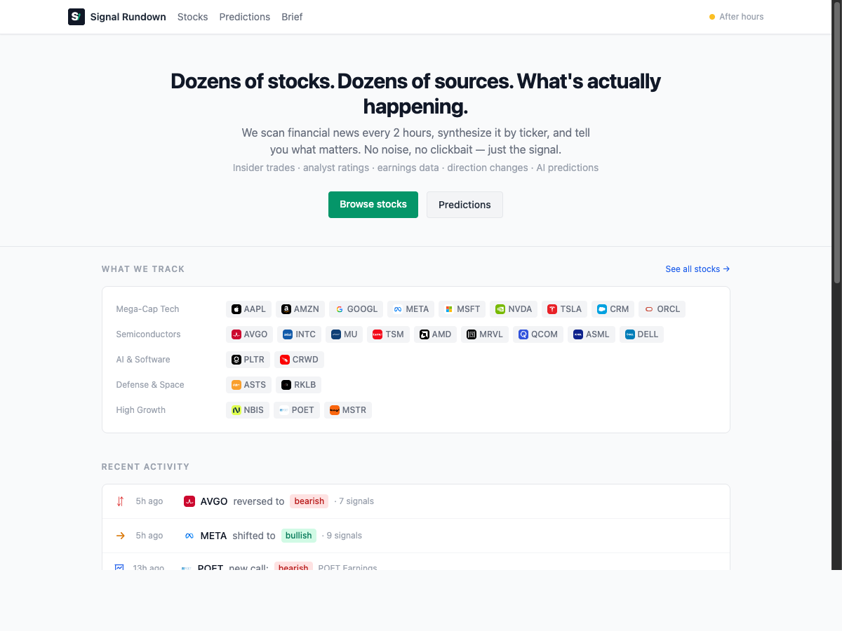
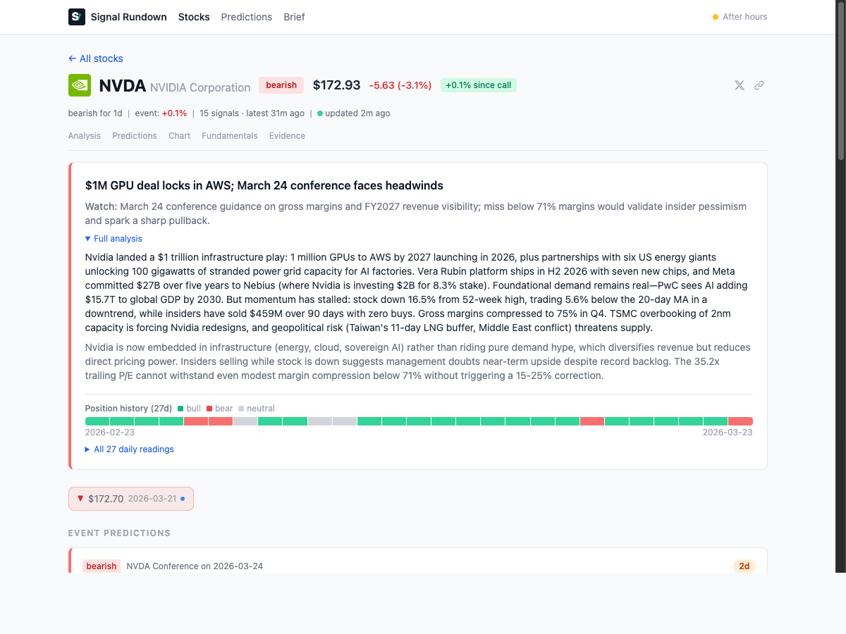
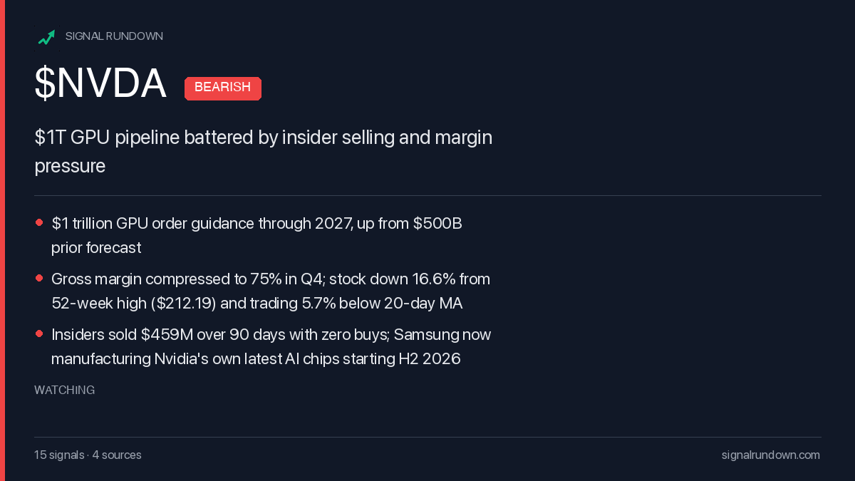
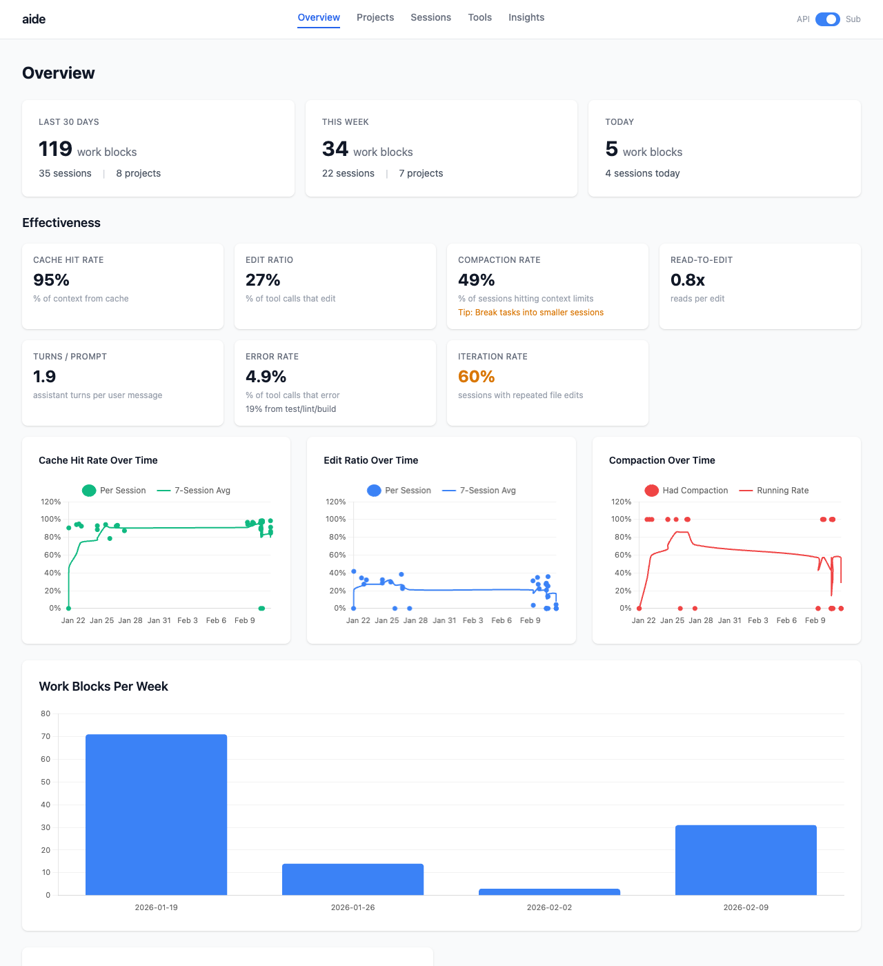
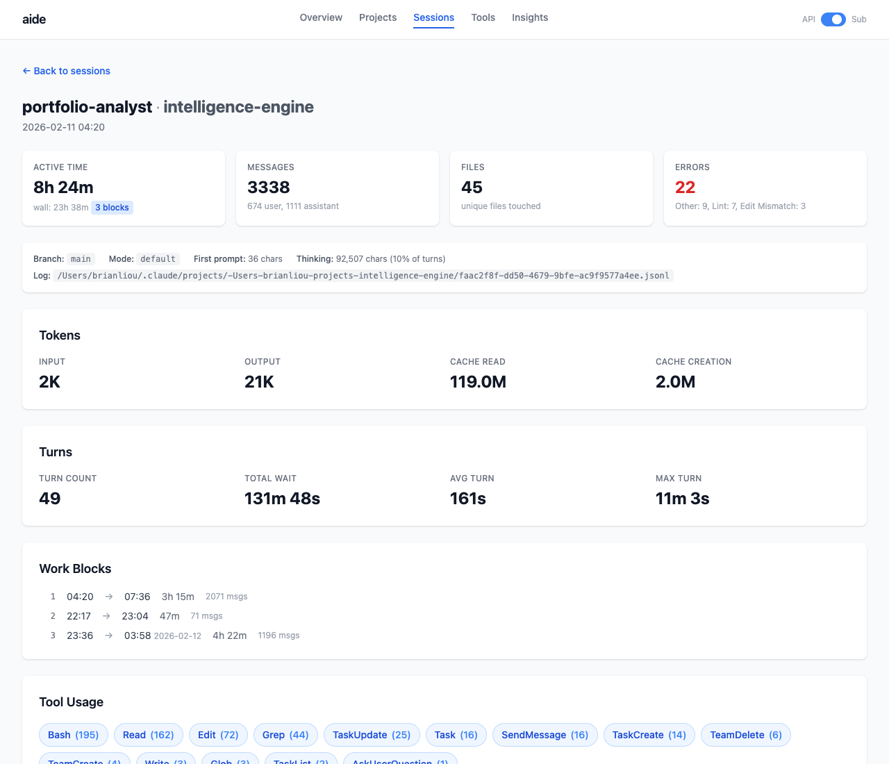
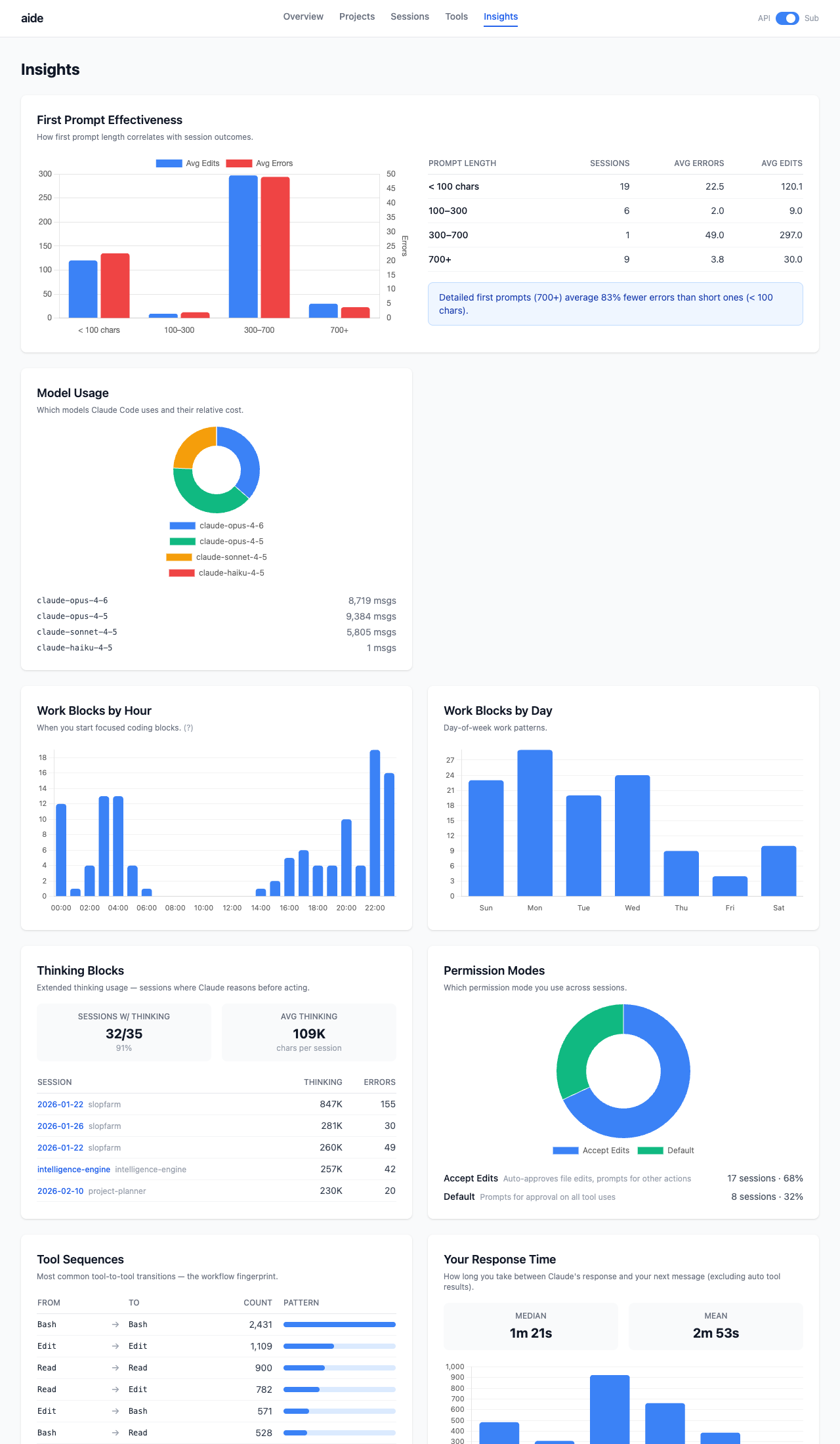
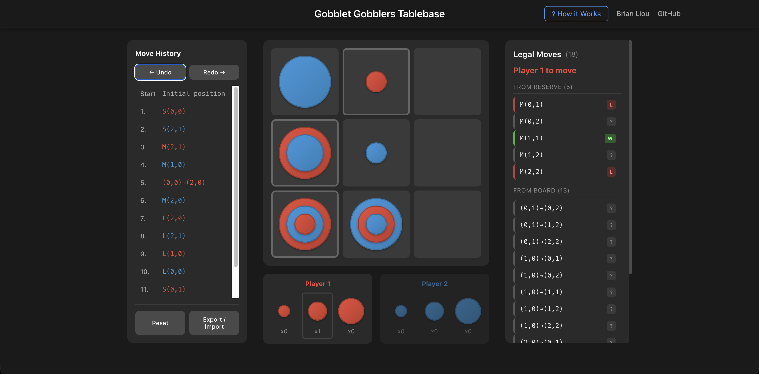 The analysis interface showing move evaluations. Green indicates winning moves, red indicates losing moves.


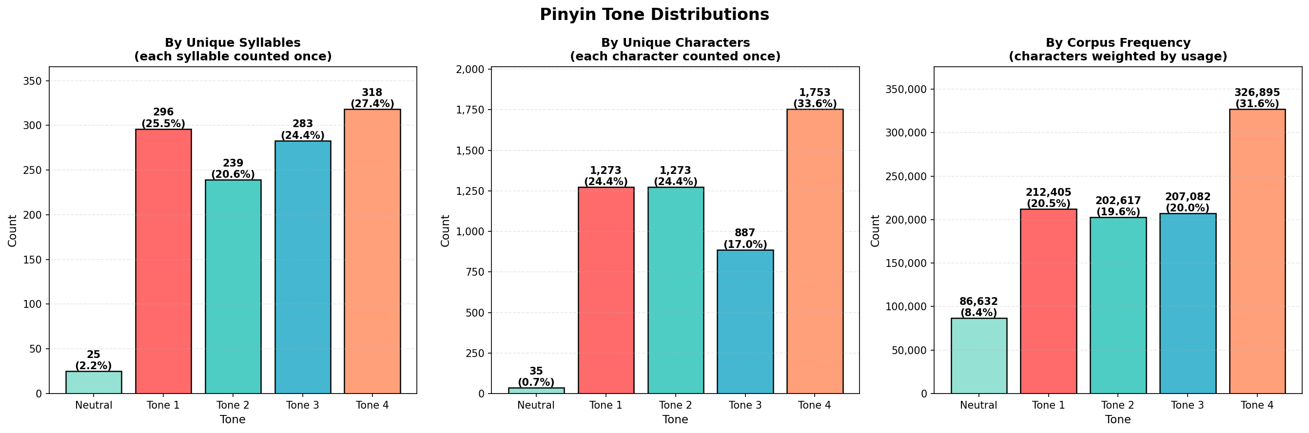 Three perspectives on tone: by syllables, by characters, and by frequency
 Character count per syllable - most have 3-4 characters, but some have 30+
 Top 20 characters with multiple pronunciations
 Syllable completion by depth - 41.5% of syllables complete at depth 4 (482 out of 1,161)
 401 base syllables × 5 tones. Cell values show character count. Some bases exist across all tones, others only in one or two.
 Prometheus showing that it’s actively scraping the API - three separate applications communicating over HTTP
 Prometheus showing time-series data - notice how it tracks changes over time
 The complete Grafana dashboard showing request rate, latency, and request distribution